Constraining cosmology with weak gravitational lensing

lessons learned from the Ultraviolet Near-Infrared Optical Northern Survey (UNIONS)

Sacha Guerrini, RHUL seminar, 8th October 2025

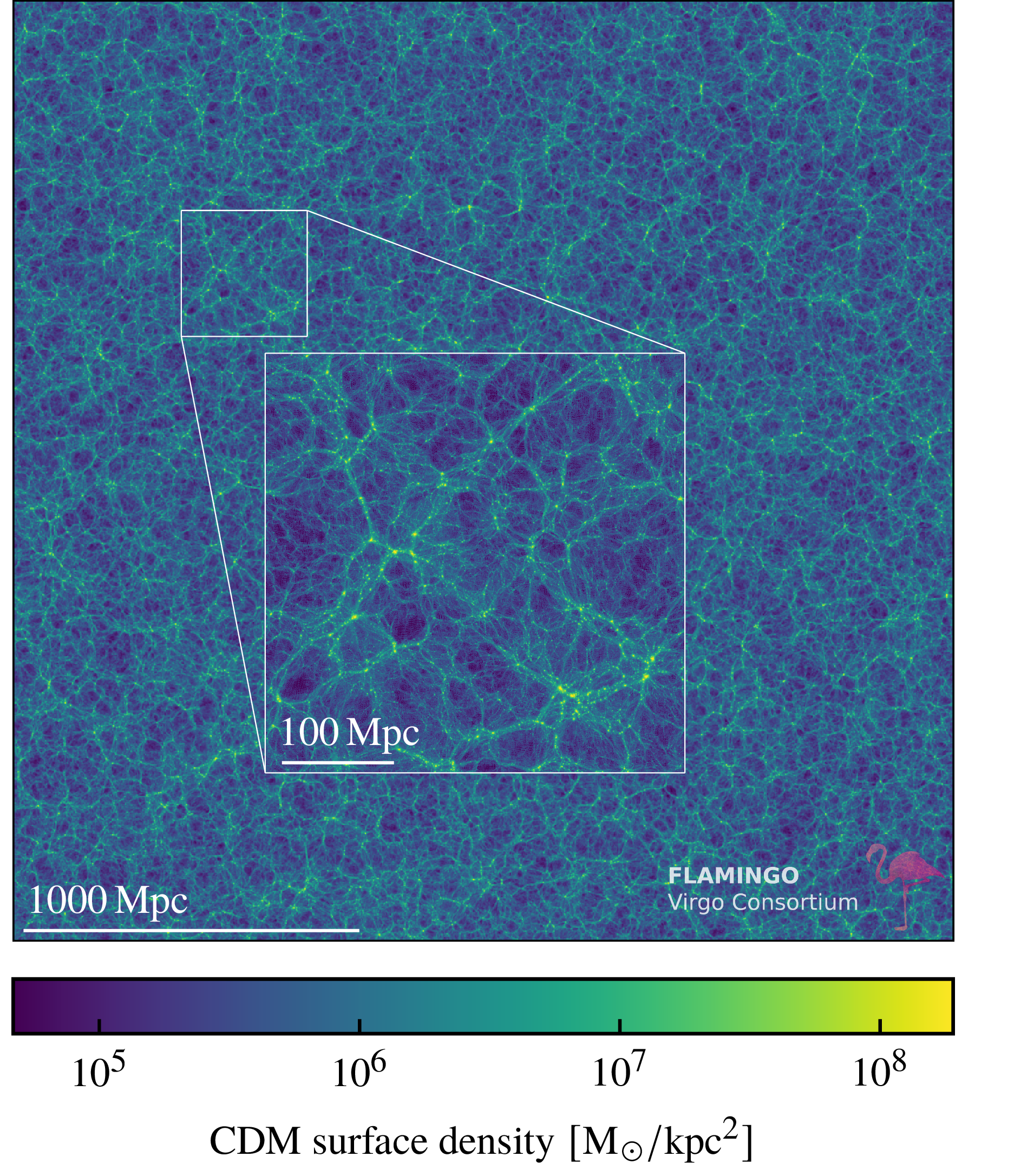
Cosmological context: \(\Lambda\)CDM

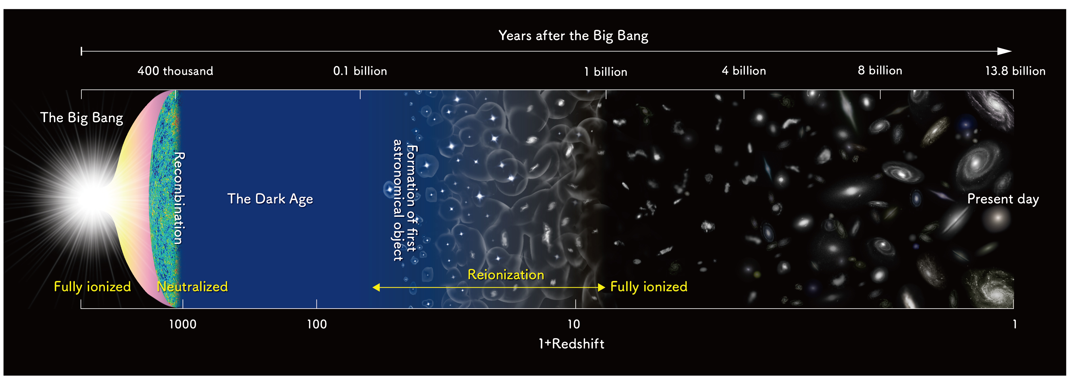
Credit: NAOJ

\[\begin{align} \left. \begin{array}{cc} H_0 & \text{Expansion rate}\\ \Omega_m & \text{Matter density}\\ \Omega_b & \text{Baryon density}\\ \sigma_8 & \text{Clumpiness}\\ w & \text{EoS of dark energy} \end{array} \right\} \text{Constrained using Bayesian inference} \end{align}\]

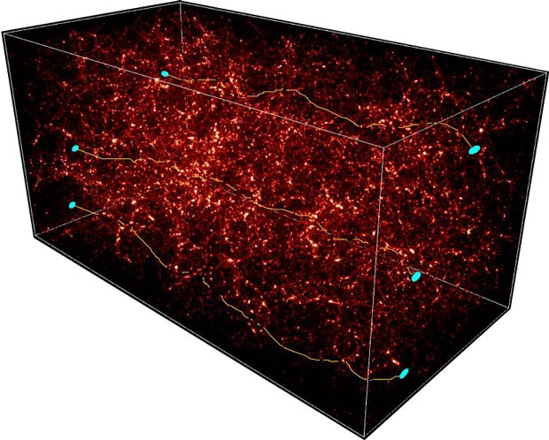
Cosmological probes and history of the Universe

Credit: NAOJ

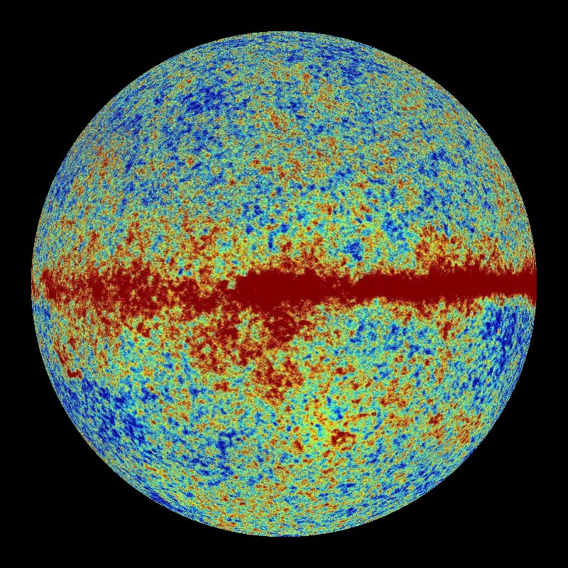
CMB

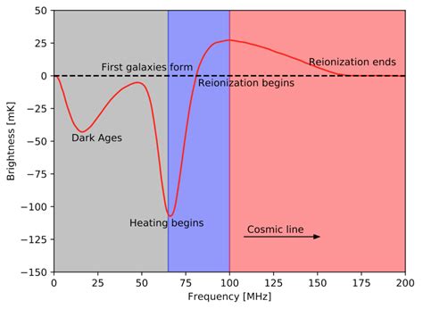
21cm/intensity mapping

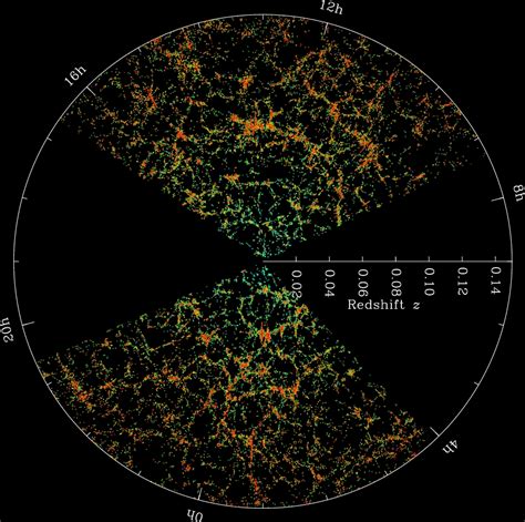
Galaxy clustering

Weak lensing

Credit: RAS

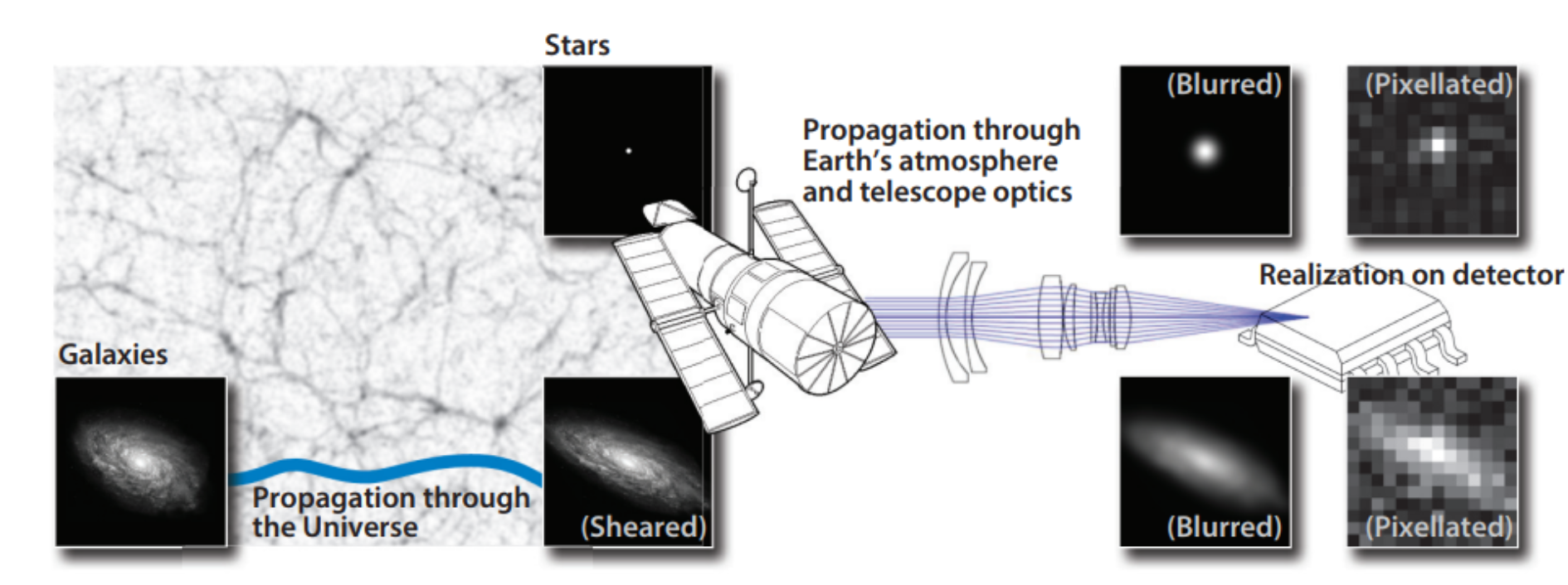
Weak gravitational lensing

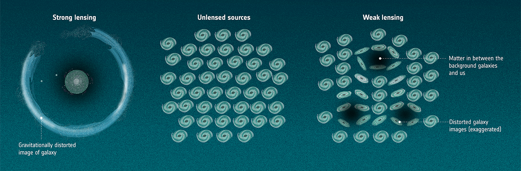
Credit: ESA

• Percent-level effect
• Polluted by shape noise
• Requires a large number of galaxies

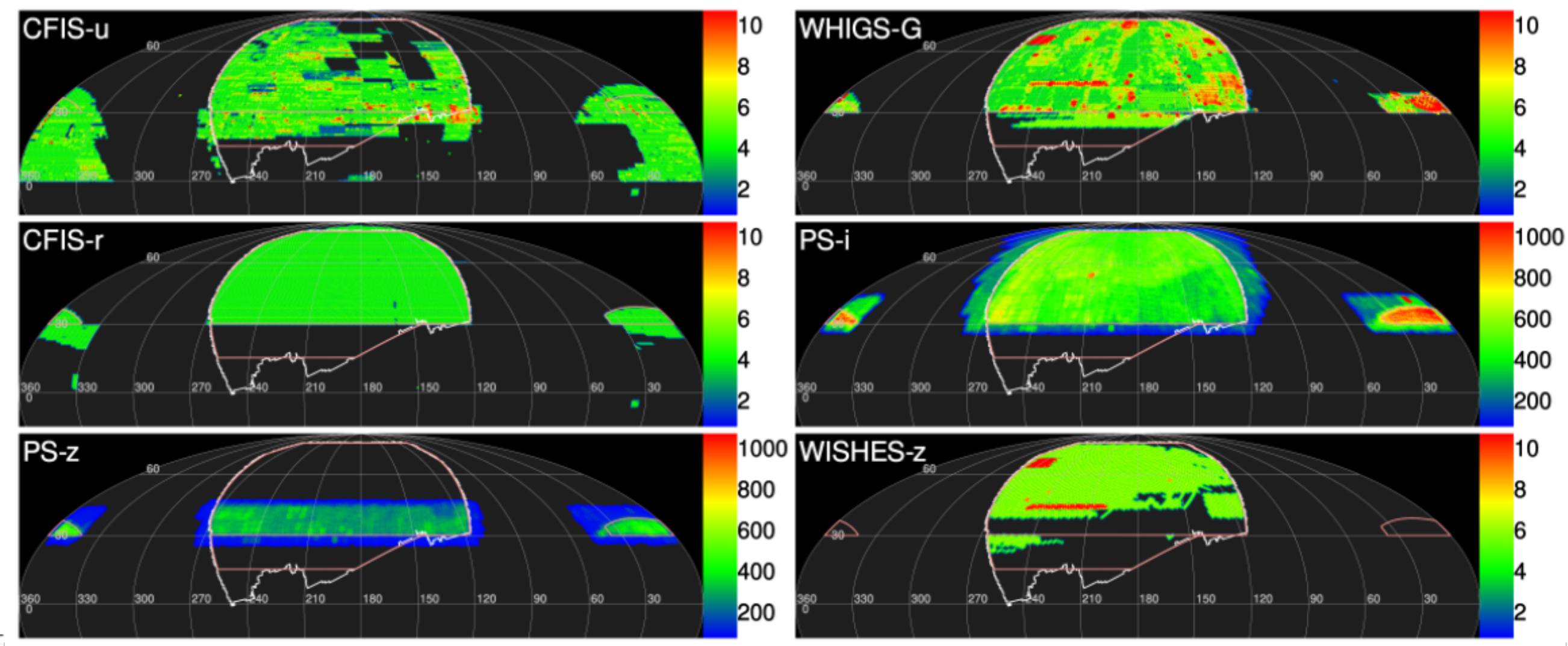
The Ultraviolet Near-Infrared Optical Northern Survey (Gwyn et al., 2025)

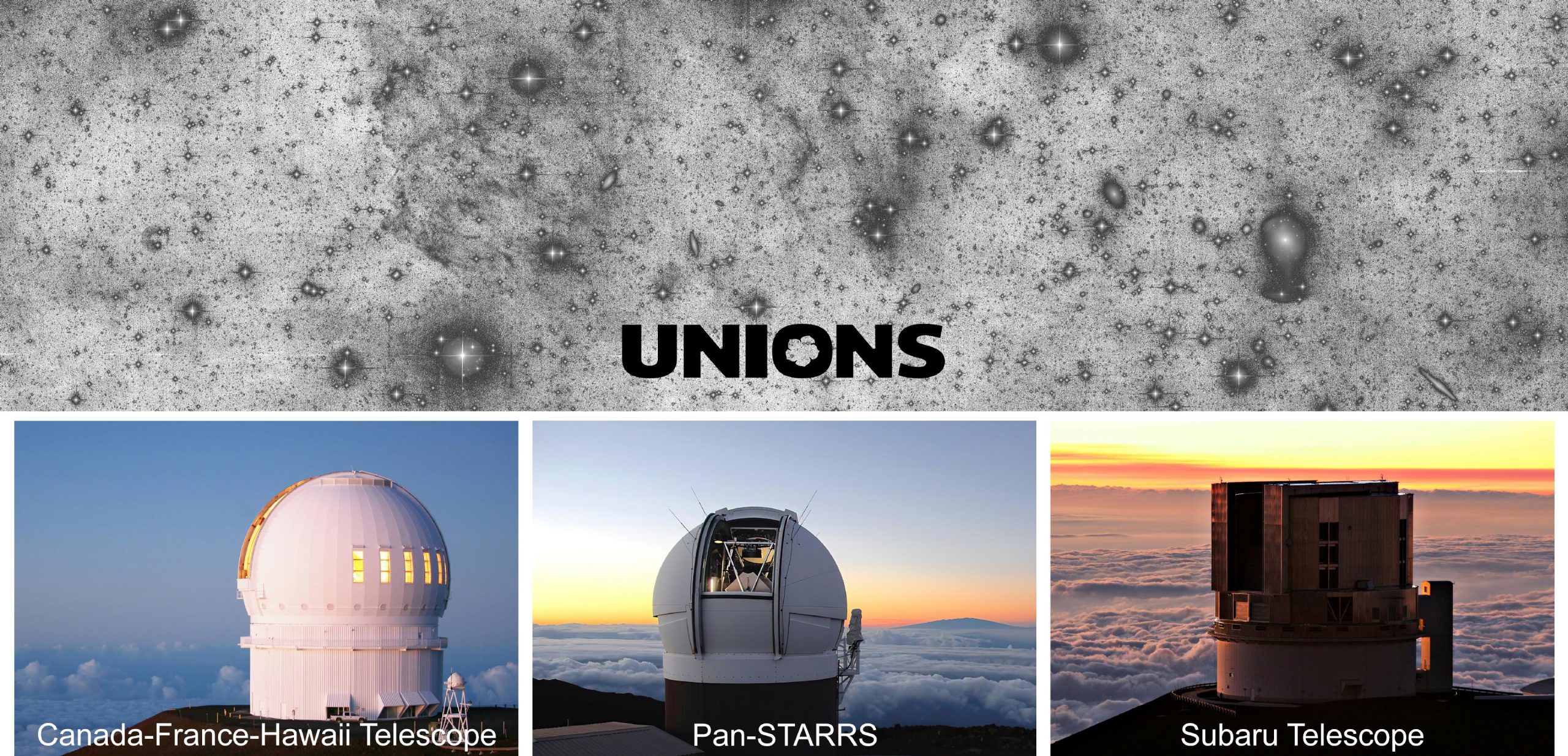
\(r\), \(u\) bands

\(i\) band

\(g\), \(z\) bands

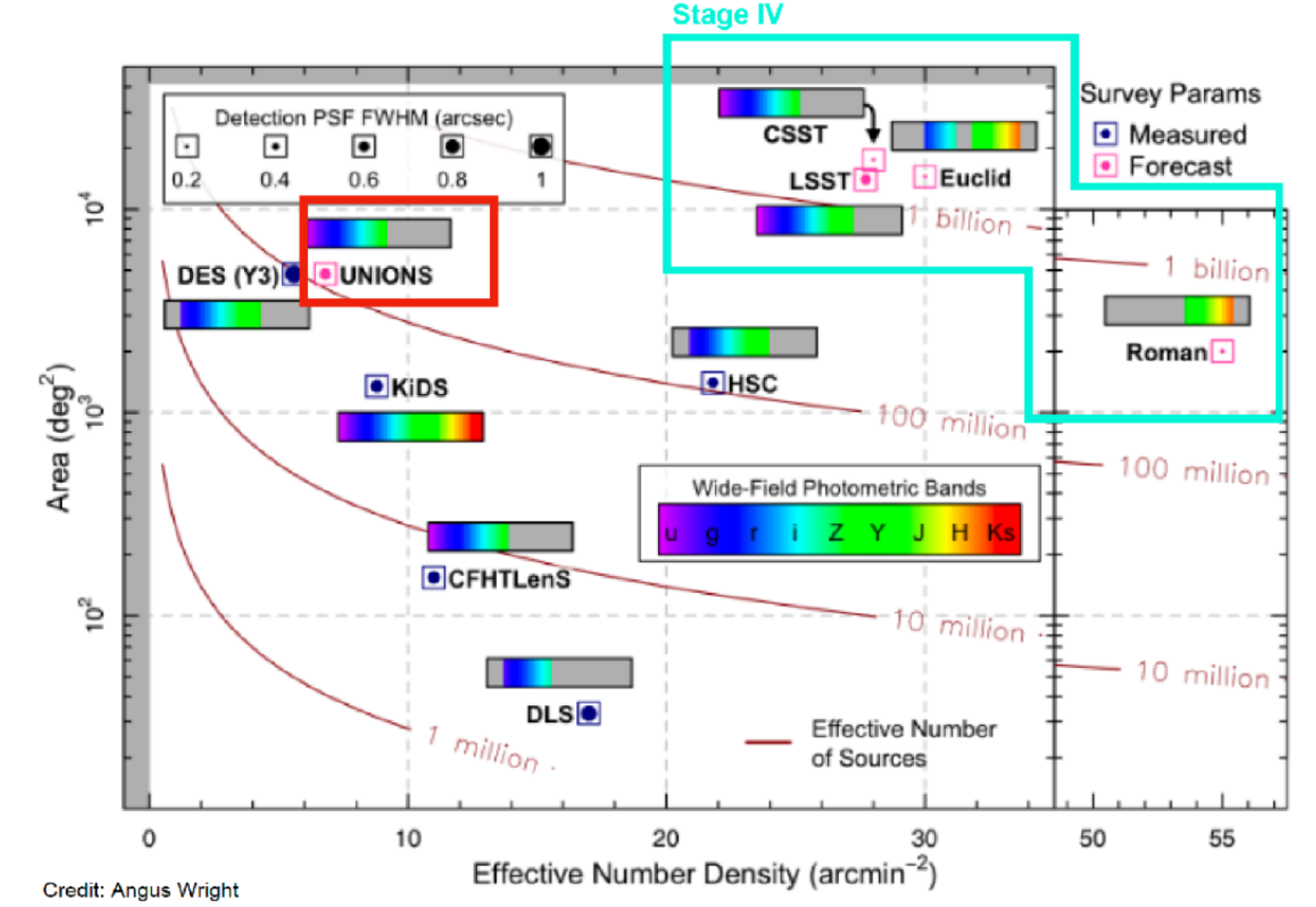
The landscape of lensing surveys

Technical specifications of UNIONS:

• Target area: \(\sim 5,000\) deg\(^2\)
• Depth: 24.5 (\(r\)-band)
• Seeing: \(\sim 0.69"\) (\(r\)-band)
• Processing with ShapePipe (Farrens et al., 2022)
• \(\sim 100\) million galaxies

Cosmology with cosmic shear

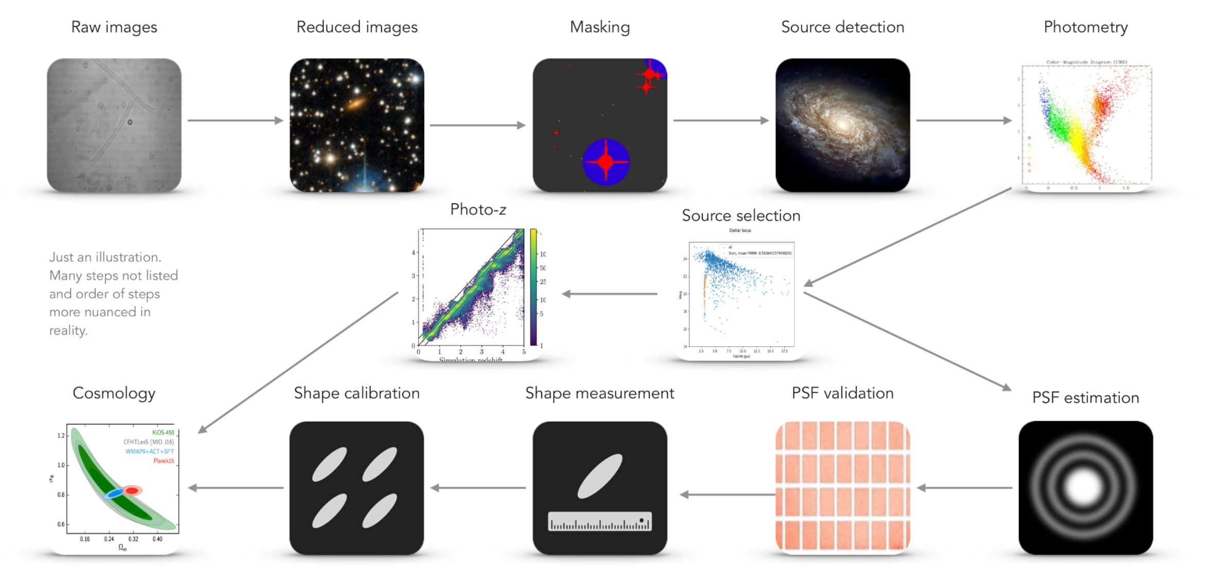
Credit: S. Farrens

I. PSF diagnostics

II. Cosmic shear with 2pt-statistics

III. And beyond

I. PSF diagnostics

Credit: Mandelbaum (2018)

PSF size error

PSF anisotropy

Credit: A. Navarro

Galaxy-PSF correlations

PSF error model: \(\delta \boldsymbol{e}^\mathrm{sys}_\mathrm{PSF} = \alpha \underbrace{\boldsymbol{e}_\mathrm{PSF}}_{\text{Leakage}} + \beta \underbrace{(\boldsymbol{e}_* - \boldsymbol{e}_\mathrm{PSF})}_{\text{Ellipticity error}} + \eta \underbrace{\boldsymbol{e}_\mathrm{PSF} \left(\frac{T_* - T_\mathrm{PSF}}{T_*} \right)}_{\text{Size error}}\). \(\alpha\), \(\beta\) and \(\eta\) free parameters.

\[\begin{equation} \left( \begin{array}{l} \tau_{0,1} \\ \tau_{2,1} \\ \tau_{5, 1} \\ \vdots \\ \tau_{0, n} \\ \tau_{2, n} \\ \tau_{5, n} \end{array} \right) = \left( \begin{array}{llllll} \rho_{0, 1} & \rho_{2, 1} & \rho_{5, 1} \\ \rho_{2, 1} & \rho_{1, 1} & \rho_{4, 1} \\ \rho_{5, 1} & \rho_{4, 1} & \rho_{3, 1} \\ & \ddots & \\ \rho_{0, n} & \rho_{2, n} & \rho_{5, n} \\ \rho_{2, n} & \rho_{1, n} & \rho_{4, n} \\ \rho_{5, n} & \rho_{4, n} & \rho_{3, n} \\ \end{array} \right) \left( \begin{array}{l} \alpha \\ \beta \\ \eta \\ \end{array} \right) \label{eq:tau_matrix} \end{equation}\]

Systematic error: \(\xi^\mathrm{sys}_\mathrm{PSF} = \alpha^2 \rho_0 + \beta^2 \rho_1 + \eta^2 \rho_3 + 2 \alpha \beta \rho_2 + 2 \alpha \eta \rho_5 + 2 \beta \eta \rho_4\)

Constrain with MCMC

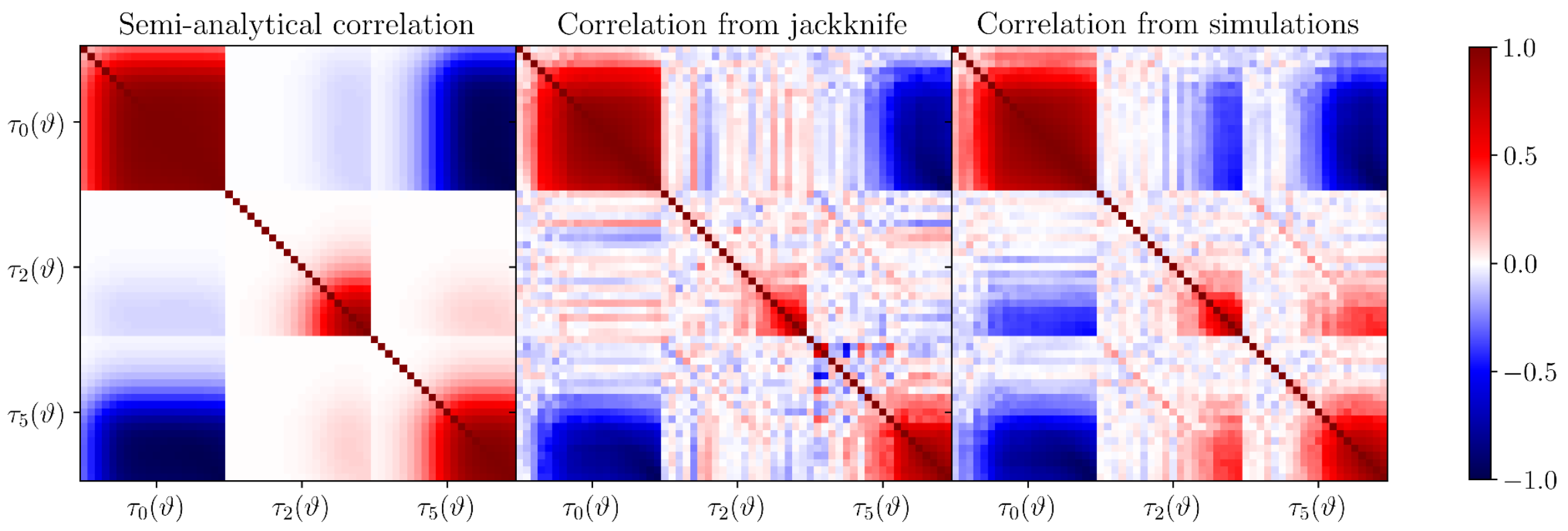
Semi-analytical covariance (Guerrini et al. (2025))

Analytical: based on analytical expressions of the covariance

Semi: No theoretical predictions of the \(\rho\)- and \(\tau\)-statistics. Use measurements on data.

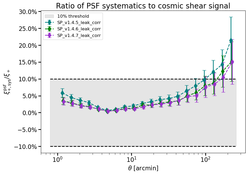
Prediction of the systematic additive bias

Estimation of PSF parameters

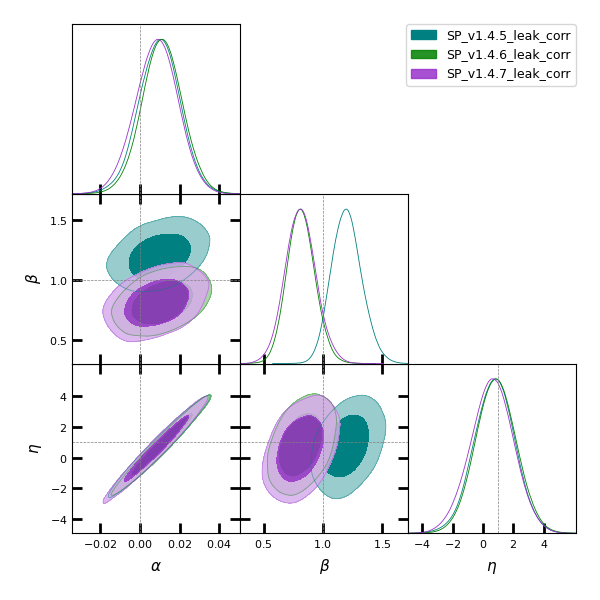
Can provide priors for cosmological analysis!

PSF systematics: Take-home messages

• PSF systematics are essential to understand to perform cosmic shear analysis.
• \(\rho\)- and \(\tau\)-statistics are powerful tools to estimate the bias to the 2PCF.
• Semi-analytical covariance (Guerrini+2025) can speed up comparisons between catalogs.

II. Cosmic shear with 2pt statistics

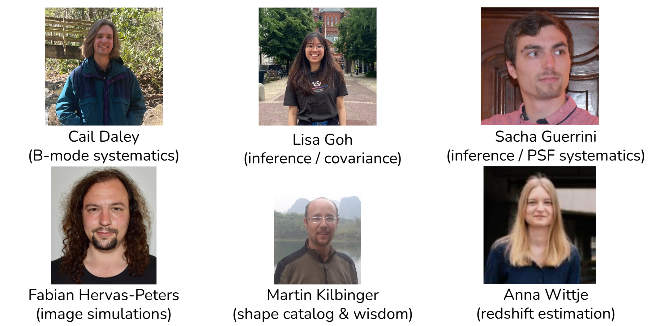
and other contributors…

Analysis details

• Theoretical prediction: CAMB
• Non-linear power spectrum: HMCode2020
• Shear calibration with MetaCalibration.
• Residual multiplicative bias estimated from image simulations. (Hervas Peters et al., in prep.)
• Cosmology pipeline with CosmoSIS.
• Analysis in real space (Goh et al., in prep.) and harmonic space (Guerrini et al., in prep.).
• PSF systematics accounted for in the inference.

Real CFHT exposure

Simulated exposure

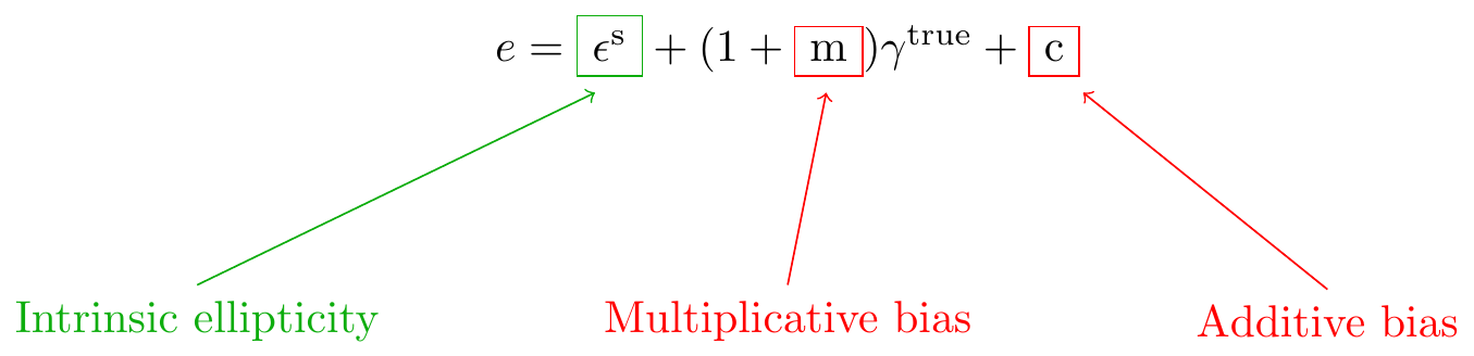
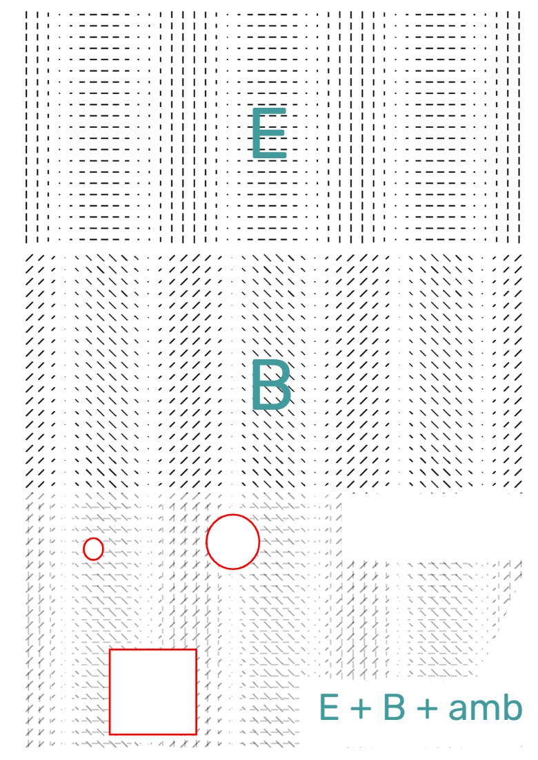
B-modes systematics

Spin-2 shear fields can be decomposed into E-modes, containing the vast majority of lensing information, and B-modes, which are a probe of systematics at UNIONS noise levels.

In the presence of masking, some ambiguous modes usually cannot be cleanly attributed to E or B.

We use three B-mode approaches: pure correlation functions, COSEBIS, and pseudo-\(C_\ell\).

Credit: BICEP2 Collaboration

Pure B-mode correlation functions

\[ \xi_+^{E/B}(\vartheta) = \frac 1 2 \left[\xi_+(\vartheta) \pm \xi_-(\vartheta) + \int_\vartheta^{\vartheta_\mathrm{max}}\frac{\mathrm{d}\theta}{\theta} \xi_-(\theta) \left(4 - \frac{12\vartheta^2}{\theta^2} \right) \right] - \frac 1 2 \underbrace{[S_+(\vartheta) \pm S_-(\vartheta)]}_{\text{Integrals of $\xi_\pm$ with filter functions}} \]

Credit: C. Daley

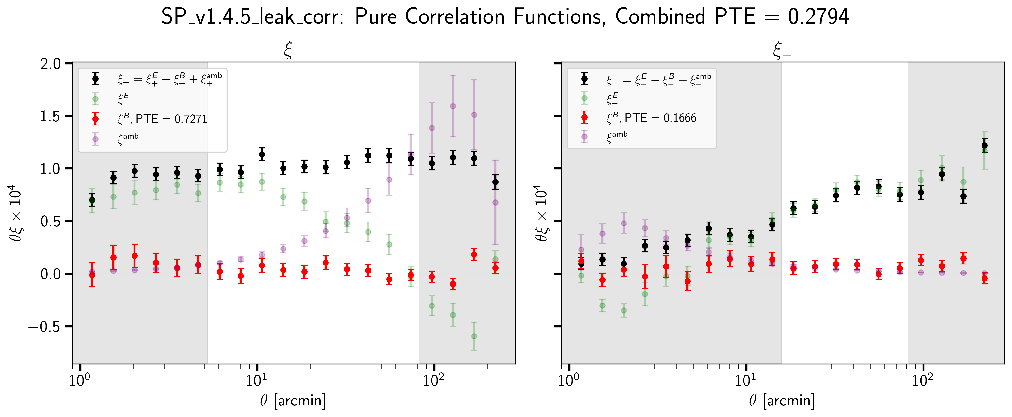
B-modes on small scale (\(\sim 3'\) in \(\xi_+\) and \(\sim 30'\) in \(\xi_-\)); large scales are ok.

B-modes with COSEBIS

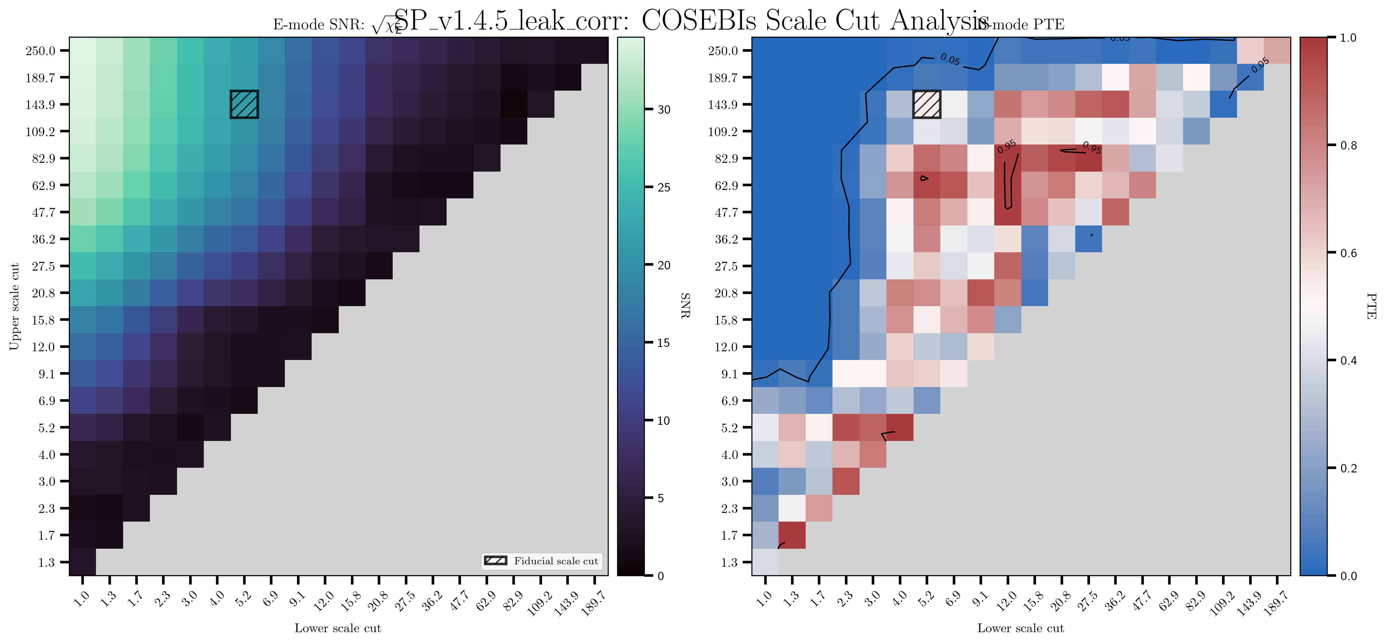
Pure functions and COSEBIS tell the same story.

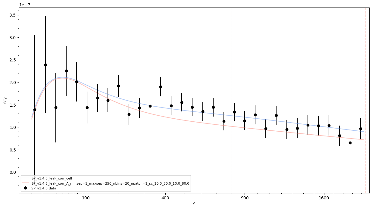
B-modes in harmonic space

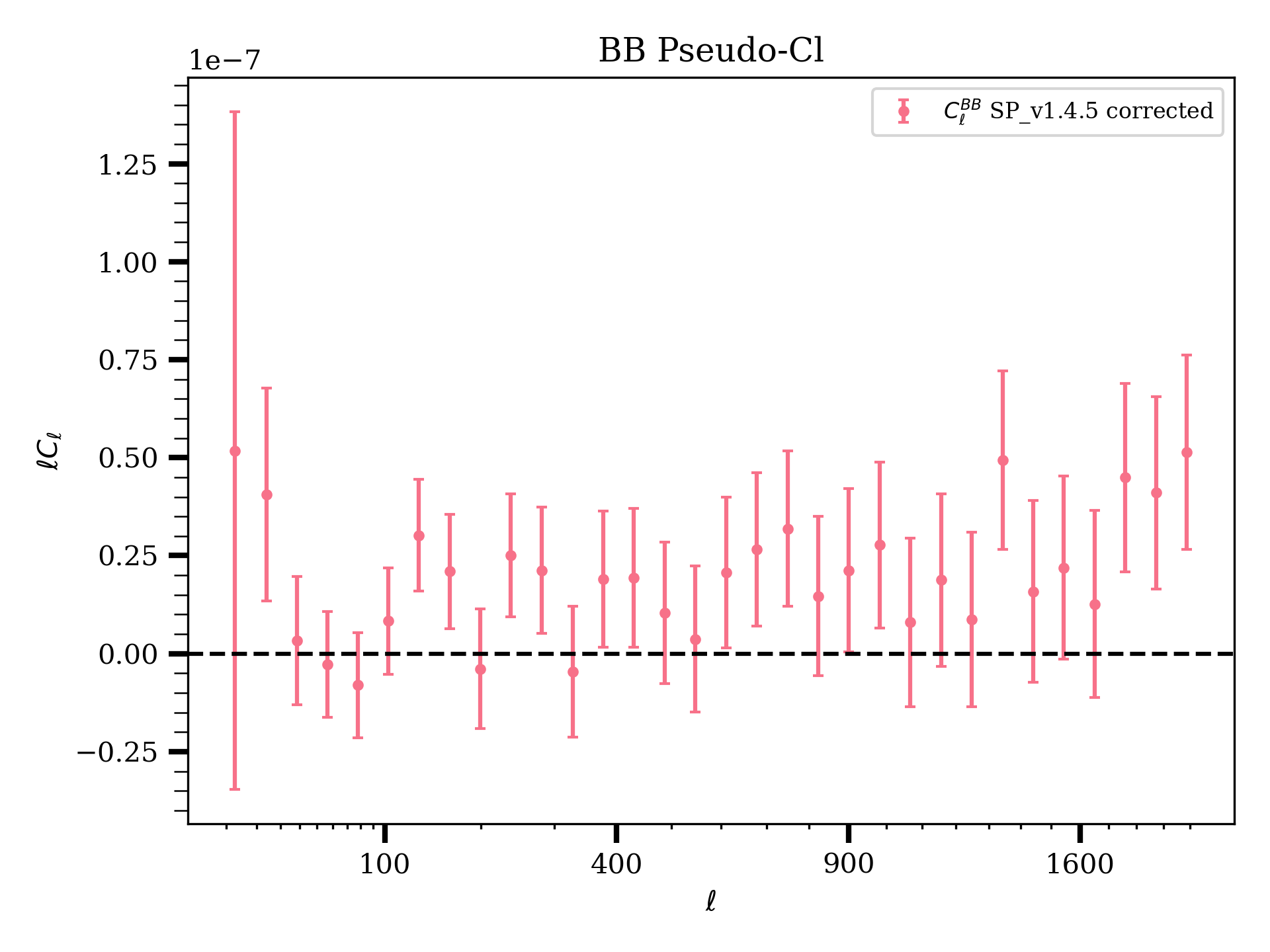
B-modes on the smallest scales. Lower significance after removing the smallest objects from the catalogue. Data points and errorbars obtained with NaMaster.

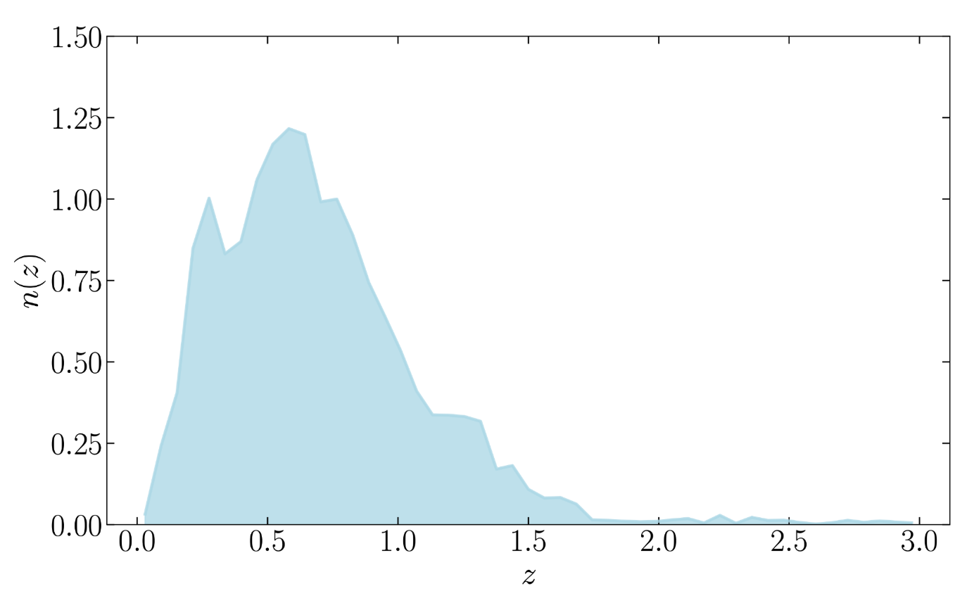
Redshift distributions

Redshift distribution estimated using self-organizing map (SOMs).

Three blinded reshift distribution produced to avoid confirmation bias. We make analysis choices given the output on the three blinds.

Credit: Anna Wittje

Covariance (real space)

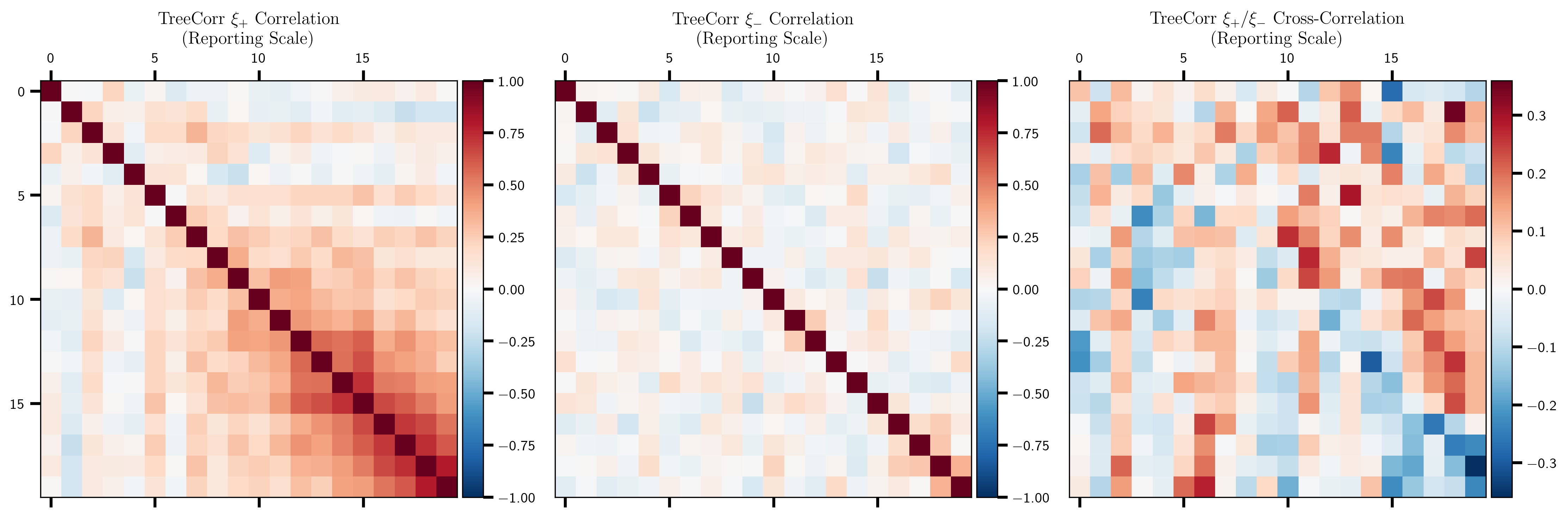
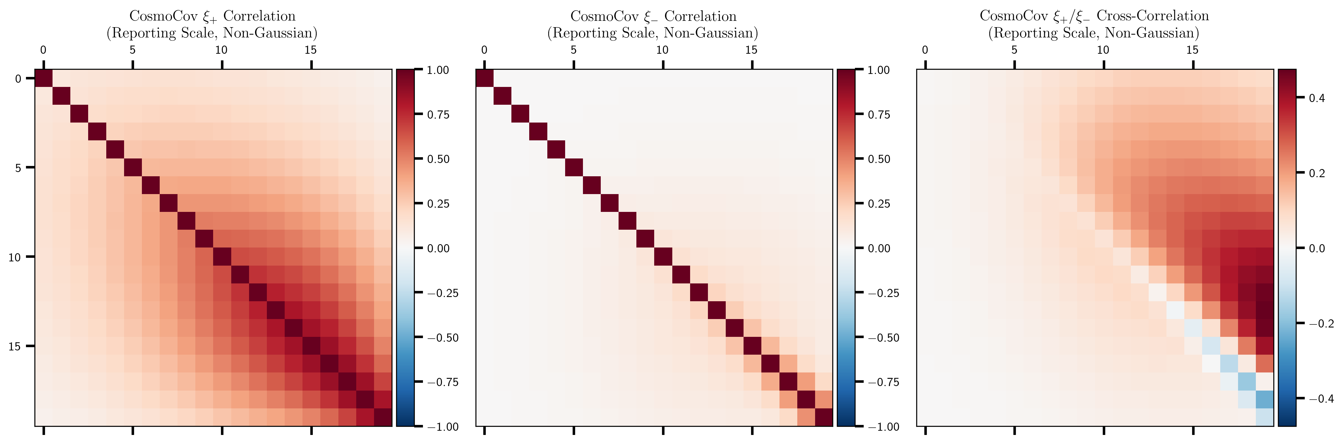
Covariance estimated with CosmoCov and validated against data-drive jackknife and GLASS simulations (not shown here).

Parameters marginalized over in inference:

• PSF systematics
• Intrinsic alignment
• multiplicative bias
• \(n(z)\) bias

Covariance (harmonic space)

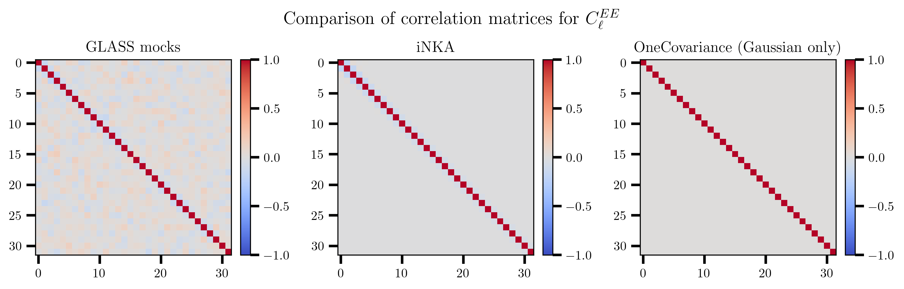
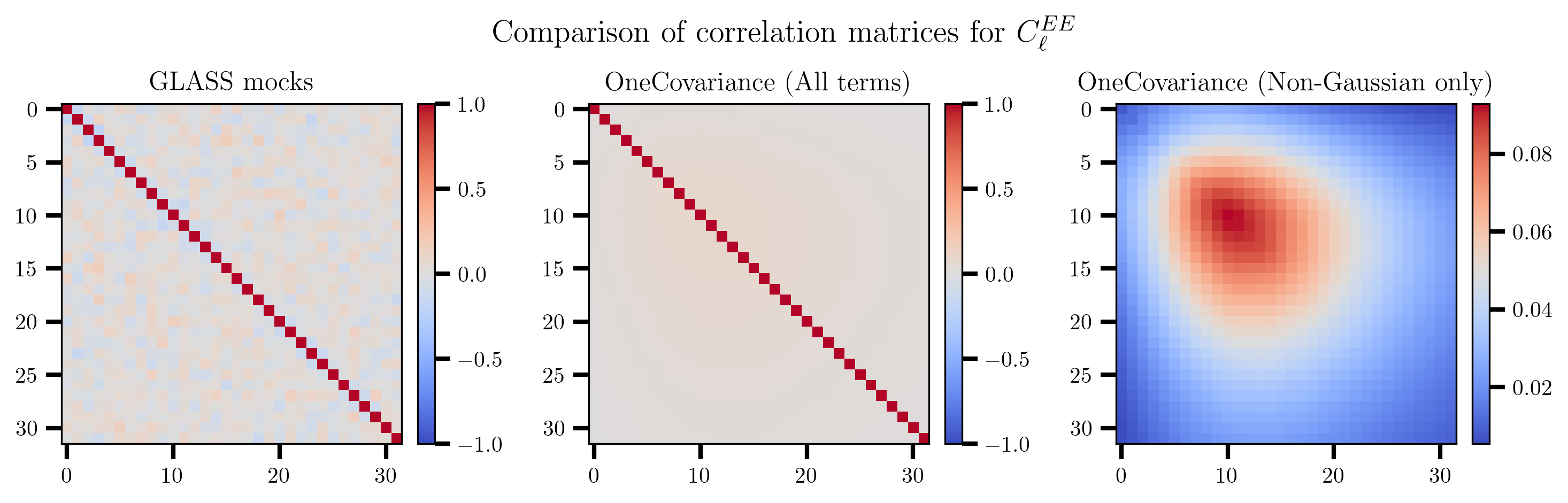
Gaussian covariance accounting for mask mode-coupling with iNKA (Namaster). Validation against OneCovariance (theory code) and GLASS mocks.

Agreement between the error bars at the \(10\%\) level

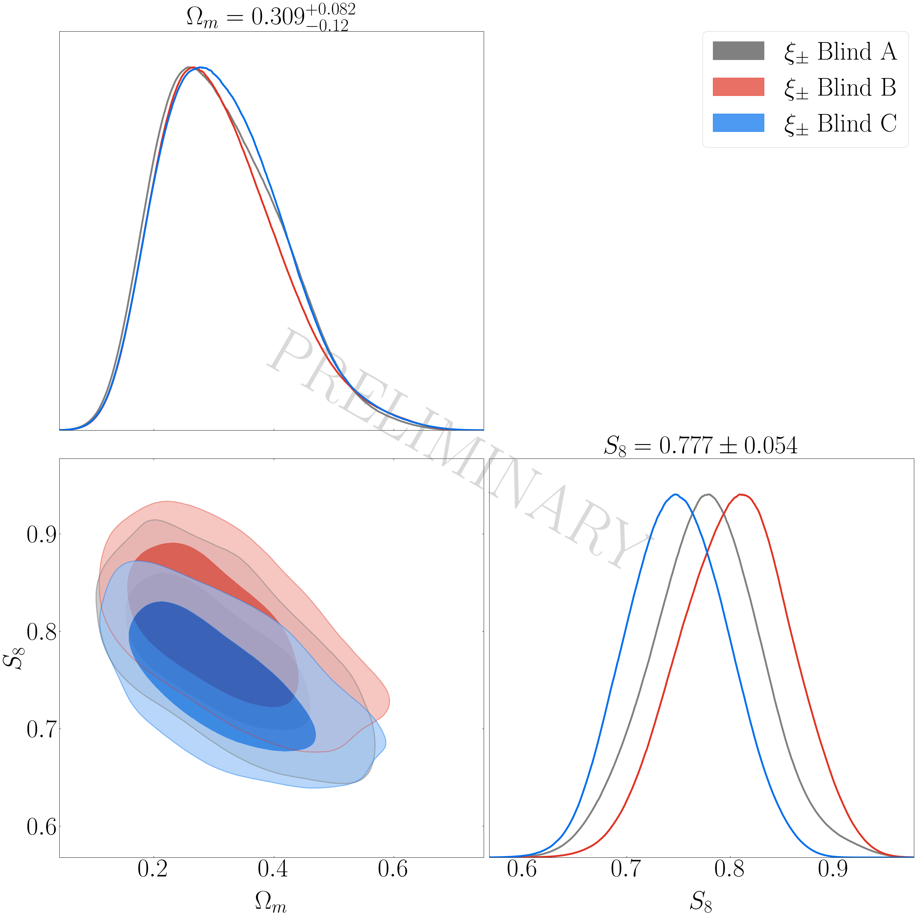
Inference

Real space \(\xi_\pm(\vartheta)\)

Harmonic space \(C_\ell\)

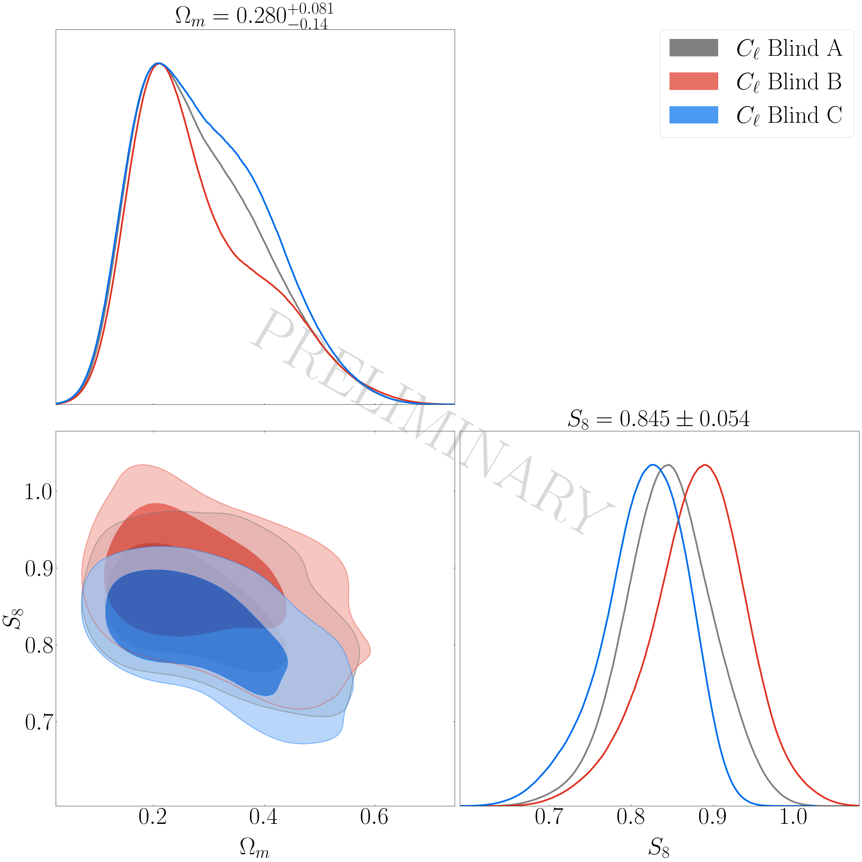
\(\sim 2\times\) larger than DES, KiDS or HSC.

Non-tomographic analysis significantly reduces constraining power.

III. Beyond 2pt statistics

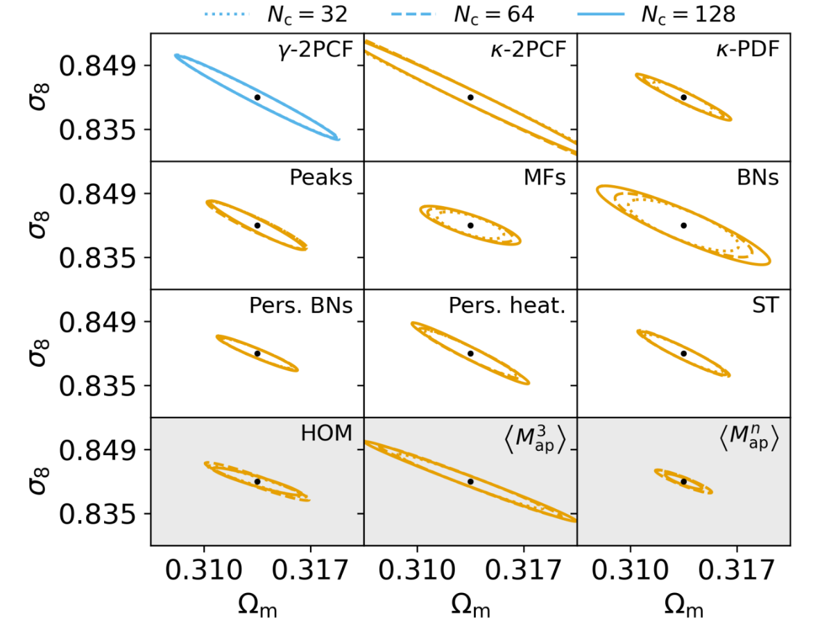
Higher-order statistics

The overdensity field is not a Gaussian field at late times.

How can we capture the more information from the shear field?

Craft summary statistics that capture non-Gaussian information from the field.

Euclid Collaboration+2023

Same methodology than 2pt?

• Does the Gaussianity of the likelihood still hold?
• Do we have a theorerical model of the higher-order summary?
• Do we know how the higher-order summary respond to systematics?

\[ p(\theta | x) \propto \underbrace{p(x|\theta)}_\text{Likelihood} p(\theta) \]

Implicit Likelihood Inference (also known as SBI)

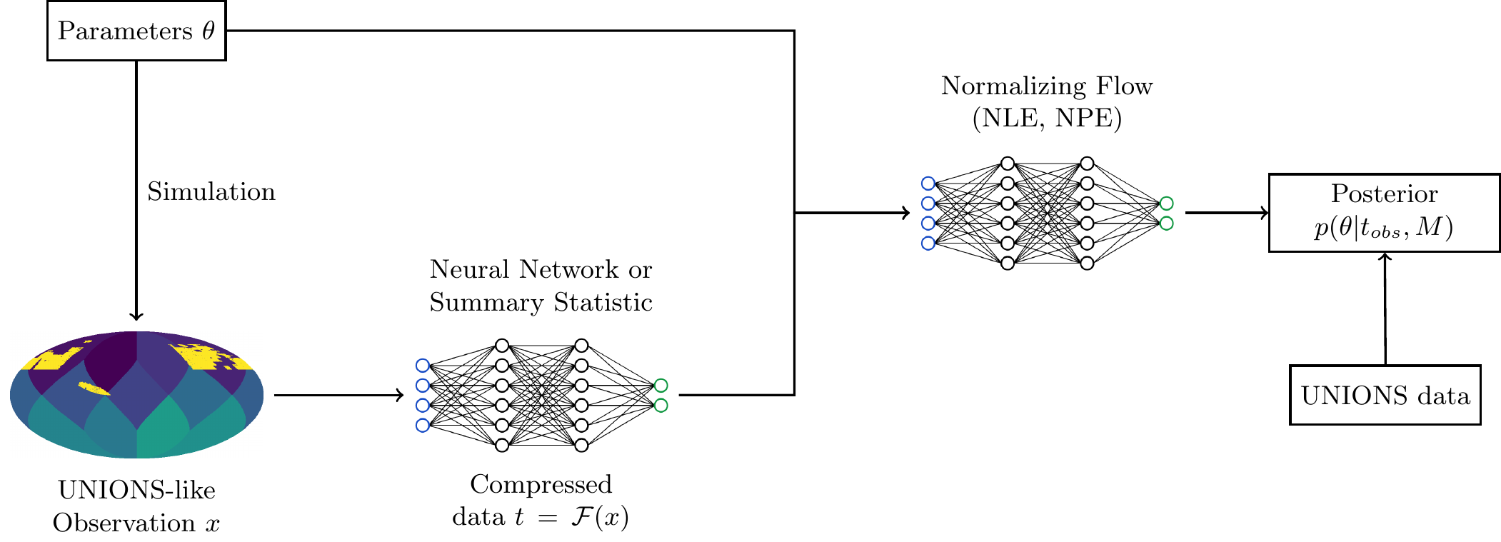
Normalizing Flows

Apply several layers of a one-to-one map to simple distribution to match a more complex one.

Alleviates the problem of the unknown likelihood.

UNIONS forward model

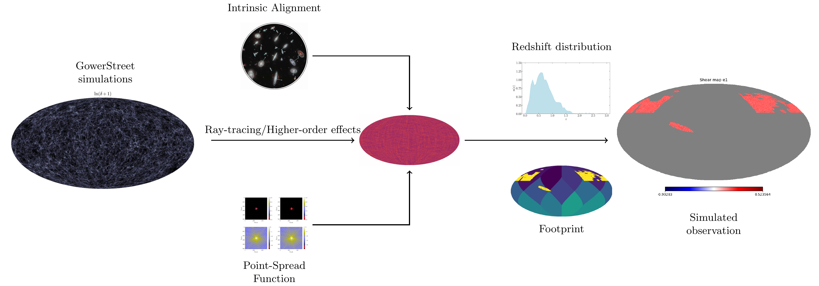
Available on GitHub

JaxILI, a pipeline for Implicit Likelihood Inference

checkpoint_path = ... #Choose the checkpoint path
checkpoint_path = os.path.abspath(checkpoint_path) #Beware, this should be an absolute path.

inference = NPE()
inference = inference.append_simulations(theta, x)

metrics, density_estimator = inference.train(
    checkpoint_path=checkpoint_path,
)

JaxILI, a pipeline for Implicit Likelihood Inference

checkpoint_path = ... #Choose the checkpoint path
checkpoint_path = os.path.abspath(checkpoint_path) #Beware, this should be an absolute path.

compressor = Compressor(
    model_class=model_class,
    model_hparams=model_hparams,
)

compressor = compressor.append_simulations(theta=theta, x=x)

metrics, MSE_compression_function = compressor.train(
    checkpoint_path=checkpoint_path
)

inference = NPE()
inference = inference.append_simulations(theta, x)

metrics, density_estimator = inference.train(
    checkpoint_path=checkpoint_path,
)

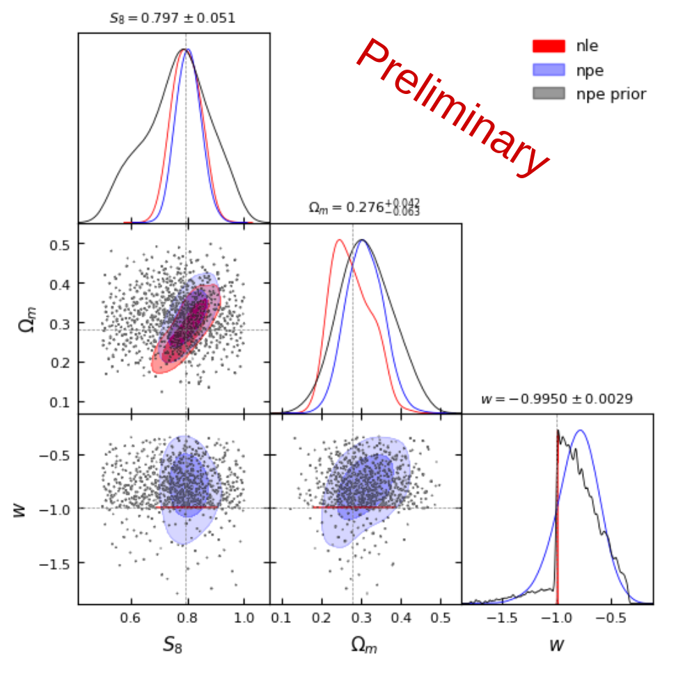
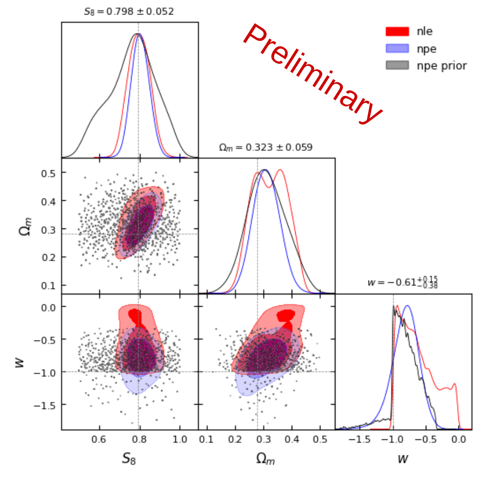
JaxILI on a cosmological toy model

Cosmological parameters: \(A_\mathrm{s}\), \(n_\mathrm{s}\), \(f_\mathrm{NL}\)

Go here for more

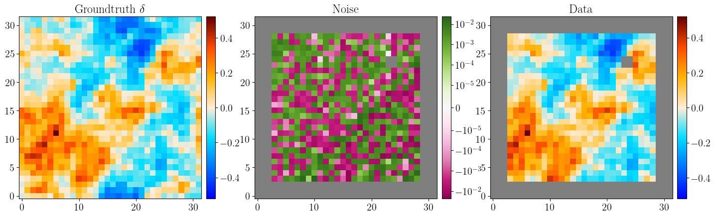
Goal: Obtain constraints on the cosmological parameters using pixel level information.

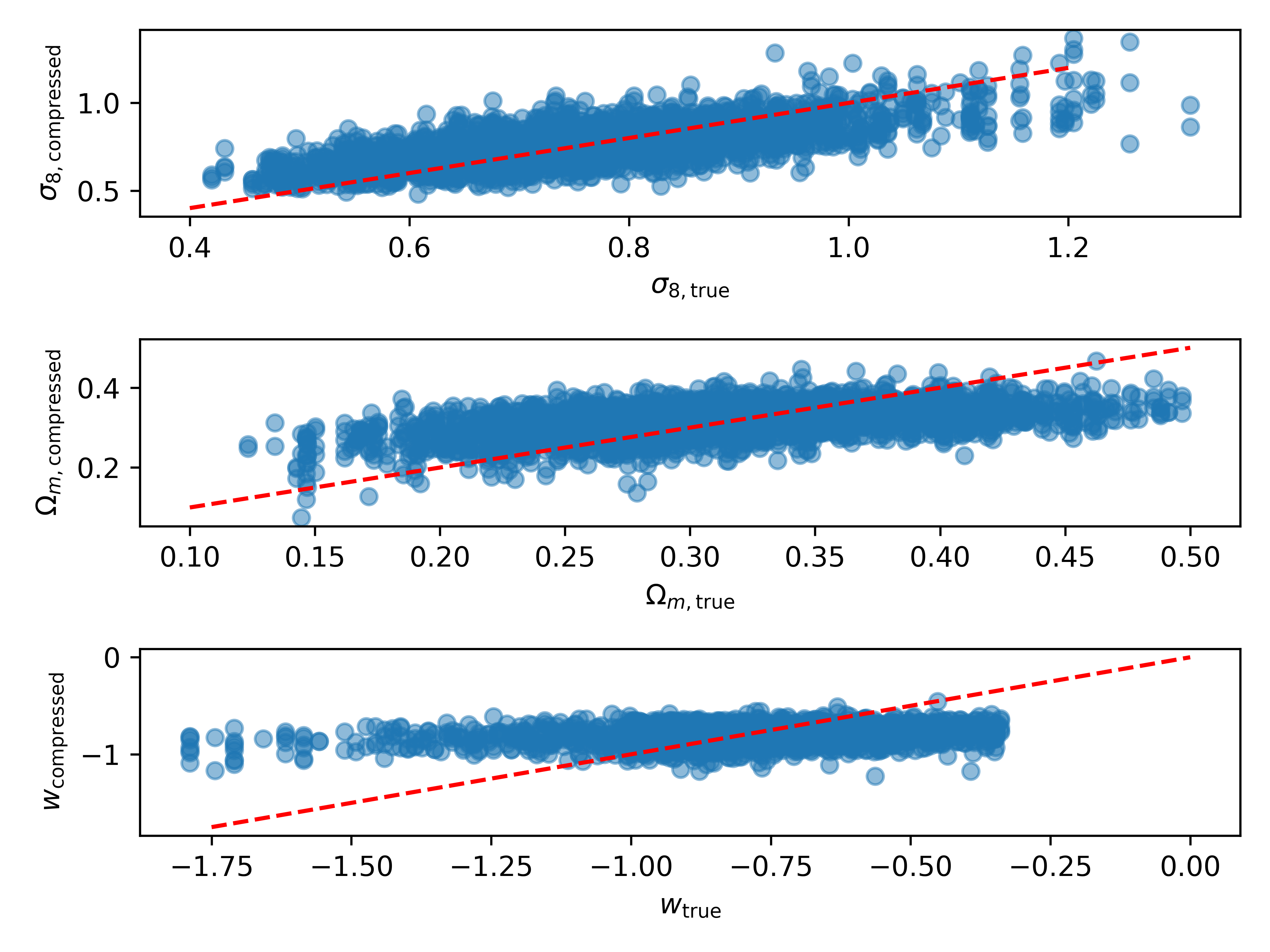
JaxILI on a cosmological toy model

Cosmological parameters: \(A_\mathrm{s}\), \(n_\mathrm{s}\), \(f_\mathrm{NL}\)

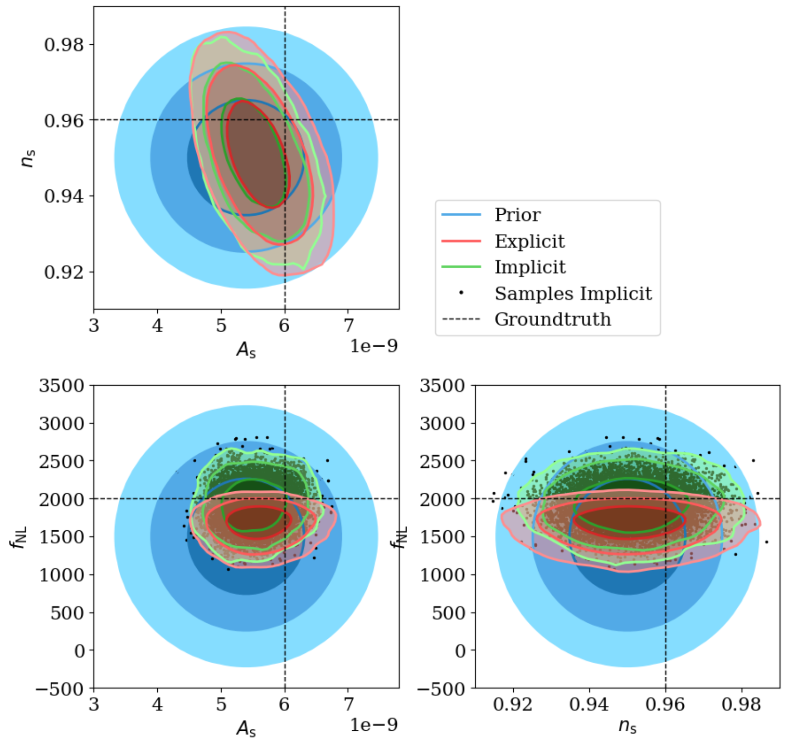
• Implicit contours obtained with MSE compression.
• Loss of information compared to Explicit inference.
• Unbiased constraints obtained.

An application of JaxILI in Euclid

Credit: R. Paviot

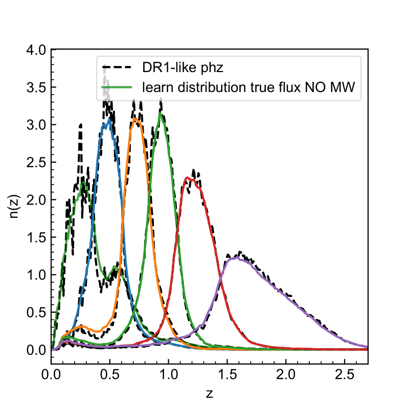
• Simulation of realistic redshift distributions using Normalizing Flow.

• \(p(z_\mathrm{noisy} | z_\mathrm{true}, \mathrm{Flux})\) infered with Neural Posterior Esimation

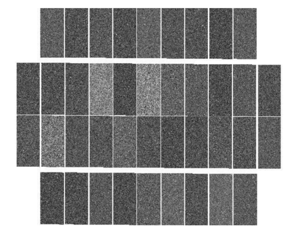
Application to UNIONS data

• CNN optimal compression
• Extract information at the pixel level.
• Cut the footprint in patches.

Credit: M. Maupas

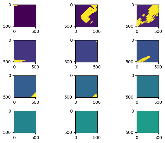
Application to UNIONS data

Conclusions

• First cosmic shear cosmology results from UNIONS are incoming!
• Allowed to develop tools used in Euclid cosmic shear analysis/validation of the data.
• Exploring advanced Bayesian inference methods to extract more information from the available datasets.

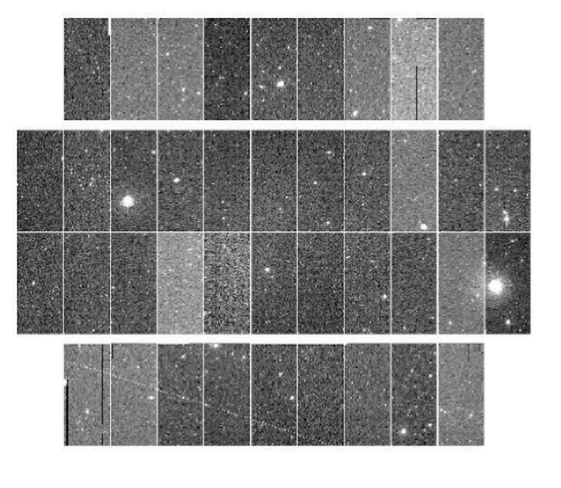
Extra material: UNIONS multi-band coverage

Extra material: MetaCalibration

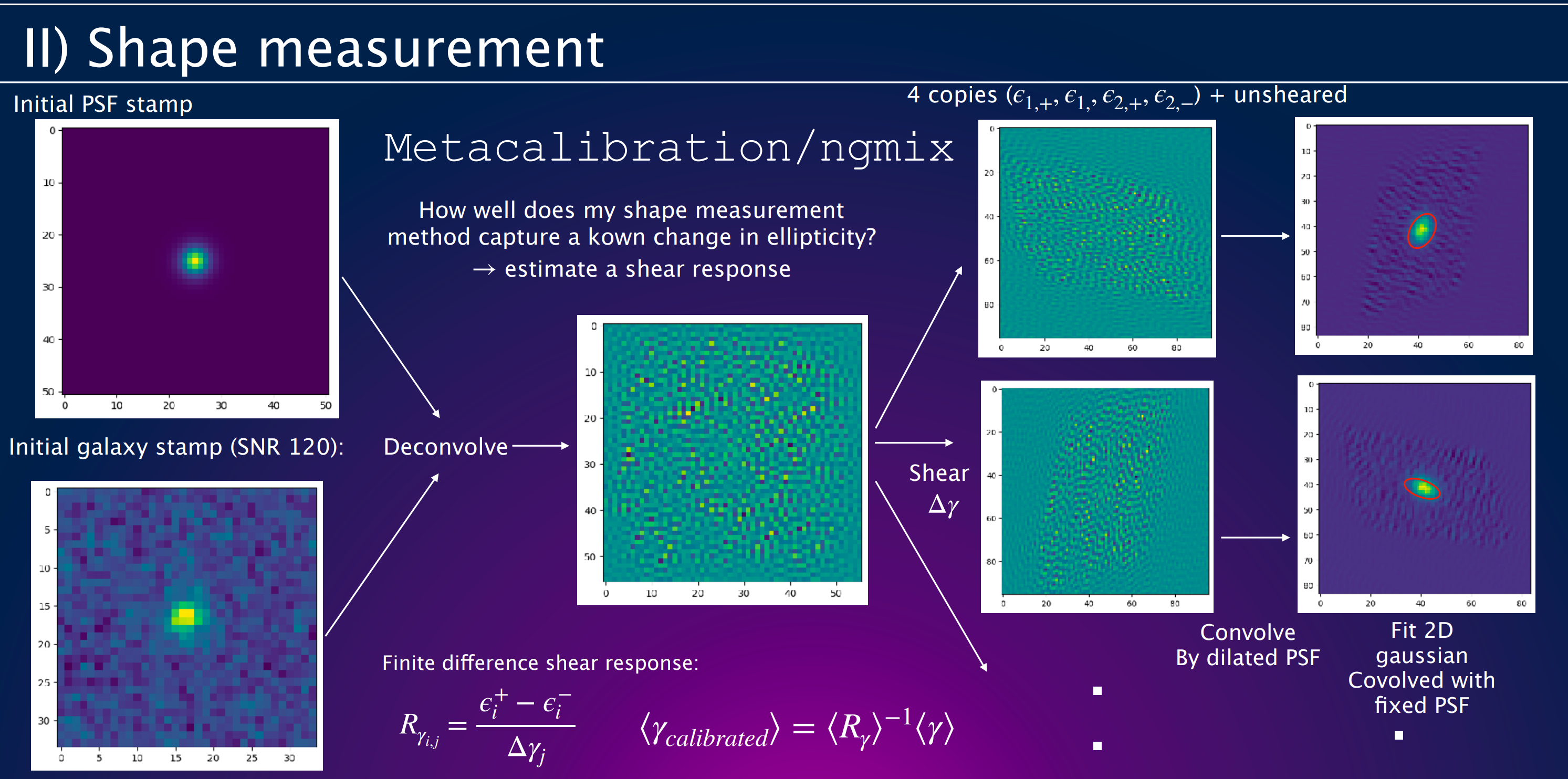
Credit: F. Hervas Peters

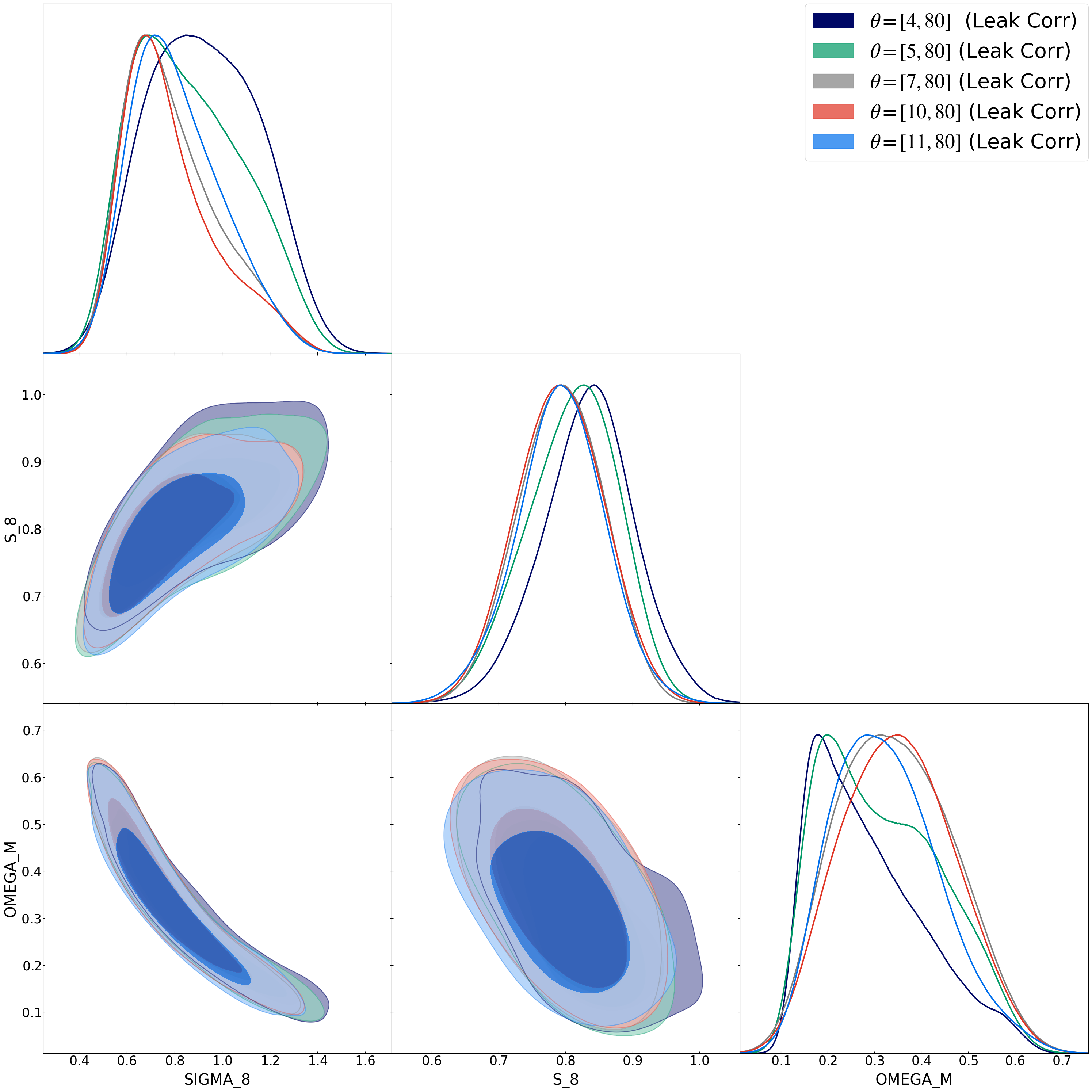
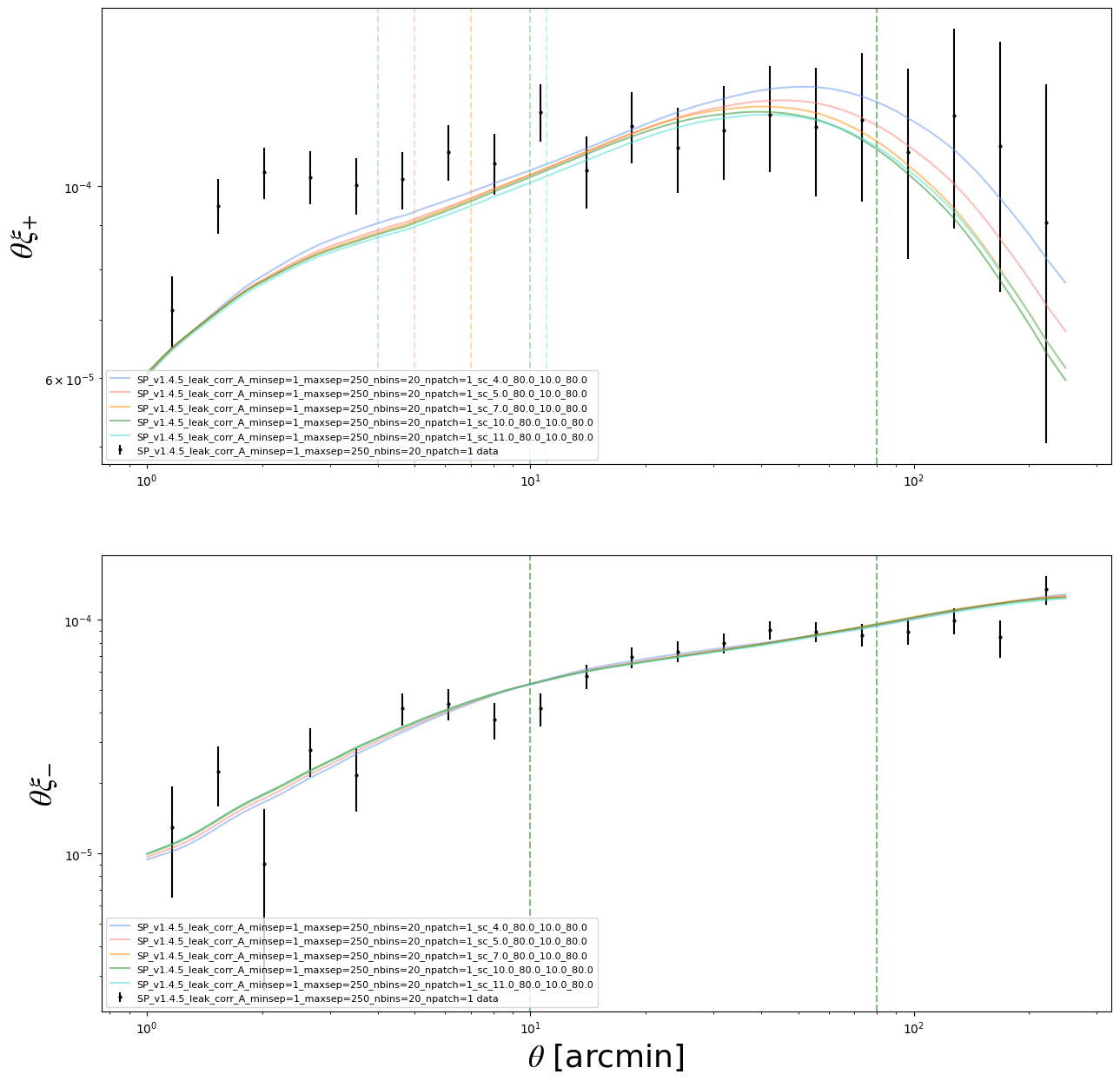
Extra material: Scale cuts

Extra material: Best-fit

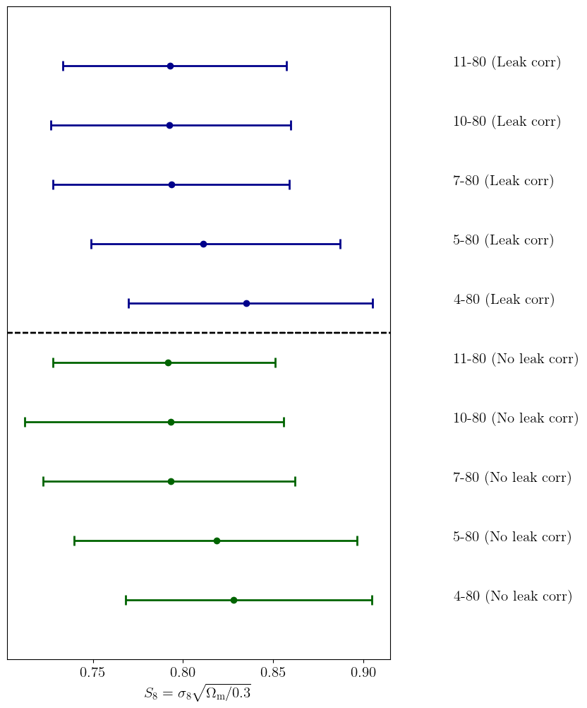
Extra material: \(S_8\) constraints

Extra material: real space vs harmonic space

Extra material: MSE compression