Field-level inference: Bayesion hierarchical model for joint field-parameter sampling
Author
Sacha Guerrini
Published
August 21, 2025
import numpy as npimport osos.environ["JAX_PLATFORM_NAME"] ="cpu"#"cpu" if you don't have access to a GPUimport urllib.requestimport jaximport jax.numpy as jnpfrom jax.scipy.stats import norm as normalimport scipy.linalg as lafrom cycler import cyclerimport matplotlib.pyplot as pltimport matplotlib.cm as cmfrom matplotlib.colors import LogNorm, SymLogNormimport matplotlib.patches as mpatchesimport matplotlib.lines as mlinesfrom mpl_toolkits.axes_grid1 import make_axes_locatableprint(f"Device used by Jax: {jax.devices()[0]}")np.random.seed(123456)
Device used by Jax: TFRT_CPU_0
Note
This document is based on a hands-on session given at Les Houches summer school 2025 on the dark universe on Field-Level Inference by Florent Leclercq. The content of this document is based on the original correction notebook and aims to go further by applying Implicit Likelihood Inference to the model introduced here.
Note on the version
This document is generated using jax and its sampling library blackjax. jax is a rapidly evolving framework. To reproduce this document, one should use the following versions of the software:
where \(\mathcal{F}\) is the Fast Fourier Transform (FFT) operator, \(T(k)\) is the transfer function, and \(D_1\) is the linear growth factor (in arbitrary units).
with shape parameter \(\Gamma = \Omega_m h \exp(-\Omega_b - \sqrt{2h}\Omega_b/\Omega_m)\). Other cosmological parameters are fixed to the following values:
Problem parameters
N =32L =1.0# box size# The following parameters will be our fiducial valuesA_s =6e-9# power spectrum normalisation, arbitrary unitsn_s =0.96# spectral indexf_NL =2000.0# non-linear coupling parameterD1 =1.732e7# growth factor of fluctuations at z=0, arbitrary units
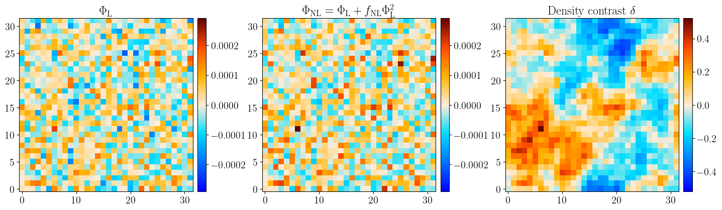
The figures below illustrate the model and the data generation process. It has been generated for fiducial parameters and will be used as observed data in what follows.
Figure 1: Visualisation of the primordial potential and the density contrast field
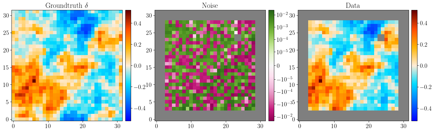
Figure 2: Visualisation of the observation. Left: the groundtruth density constrast, Middle: the mask and noise matrix, Right: the observed data.
Inferring the parameters using the field
Using Bayesian inference, we want to estimate the parameters \(\boldsymbol{\theta} = (A_\mathrm{s}, n_\mathrm{s}, f_\mathrm{NL})\) given the data \(d\) and the noise variance field \(N\).
Here our data \(d\) is the observed field, hence the name field-level inference. In the previous section, we have build a Bayesian Herarchical Model (BHM) for the data, which specifies the likelihood.
However, the likelihood is defined at the pixel level. We have access to \(p(\boldsymbol{\theta}, z | d)\) where \(z\) are the primordial pixel values. In practice, to get constraints on the cosmological parameters only, we must marginalise on pixel values \(z\).
This integral is intractable in practice. Sampling cosmological parameters and initial conditions is a challenging task as the problem is very high dimensional. It requires sampling techniques that are not sensitive to the curse of dimensionality such as Hamiltonian Monte Carlo.
A first task is to write the log-prior, log-likelihood and log-posterior functions for the BHM.
We can summarise the model using the following diagram:
flowchart TD
  A(("$$A_\mathrm{s} \sim \mathcal{N}(\mu_{A_\mathrm{s}}, \sigma_{A_\mathrm{s}})$$")) --> C["$$P(k)$$"]
  B(("$$n_\mathrm{s} \sim \mathcal{N}(\mu_{n_\mathrm{s}}, \sigma_{n_\mathrm{s}})$$")) --> C
  C --> D(("$$\Phi_\mathrm{L} \sim \mathcal{N}(0, P(k))$$"))
  D --> F["$$\Phi_\mathrm{NL}$$"]
  E(("$$f_\mathrm{NL} \sim \mathcal{N}(\mu_{f_\mathrm{NL}}, \sigma_{f_\mathrm{NL}})$$")) --> F
  F --> G["$$\delta$$"]
  G --> I["$$d$$"]
  H(("$$n \sim \mathcal{N}(0, N)$$")) --> I
  I <--> J[observation]
Figure 3: Bayesian hierarchical model for field-level inference. Round boxes are sampled from and rectangular boxes are derived.
In what follows, we will use the following values for the prior of the cosmological parameters. The likelihood is explicitely defined via the choices of distribution from which the parameters (prior) and latent variables are sampled from. Probabilistic programming languages such as pyro or numpyro implement BHMs following the graph structure sketched in Figure 3.
# Define hyperparameters for the priorA_s_scale =6e-9f_NL_scale =2e3mu_A_s =0.9* A_s_scalesigma_A_s =0.1* A_s_scalemu_n_s =0.95sigma_n_s =0.01mu_f_NL =0.75* f_NL_scalesigma_f_NL =0.25* f_NL_scale
The output of the log-prior, log-likelihood and log-posterior functions is a scalar value and can be found for various examples below.
# Test the functions with the ground truth white noise fieldtheta = pack_theta(A_s=A_s, n_s=n_s, f_NL=f_NL, field=white_noise)log_prior(theta), log_likelihood(theta, data, noise_variance_field), log_posterior( theta, data, noise_variance_field)
# Generate a new white noise field and compute the log-likelihoodwhite_noise_2 = jax.random.normal(jax.random.PRNGKey(2), (N, N))theta_2 = pack_theta(A_s=A_s, n_s=n_s, f_NL=f_NL, field=white_noise_2)log_likelihood(theta_2, data, noise_variance_field), log_prior(theta_2), log_posterior( theta_2, data, noise_variance_field)
Sample the posterior using field-level inference (explicit)
To efficiently sample parameters in a high-dimensional space, one must rely on gradient-based Markov Chain Monte Carlo (MCMC) techniques such as HMC. jax is a powerful library that uses autodiffertiation to compute gradient of functions in such a way that, given the log-likelihood function is written in jax, we have access to it for free.
In what follows, we use the No-U-Turn Sampler (NUTS) from the blackjax library, which is a JAX implementation of the NUTS algorithm to sample the cosmological parameters and the initial conditions of the field at the same time. jax can run automatically on GPU. In this document, we ran on CPU on a laptop and sampling five chains of \(10,000\) samples each takes around two hours. I have not checked the speed up obtained by running on GPU.
It is possible to speed up the sampling by using Gibbs sampling to sample the field with HMC and the cosmological parameters with e.g. slice sampling. The implementation of it currently does not perform correctly. In what follows, diagnostics of the chains will be presented using the NUTS algorithm.
Why is it more efficient that way?
Diagnose the chains
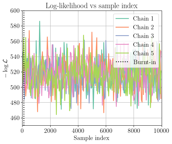
Log-likelihood
Figure 4: Log-likelihood trace plot for each chain. The dashed line indicates a burn-in period of a hundred samples.
Trace plots
We can then check the trace plots for parameters such pixels and cosmological parameters.
Figure 5: Trace plots for the pixel values at (10, 20) and (25, 10) for each chain. The dashed line indicates the groundtruth value.
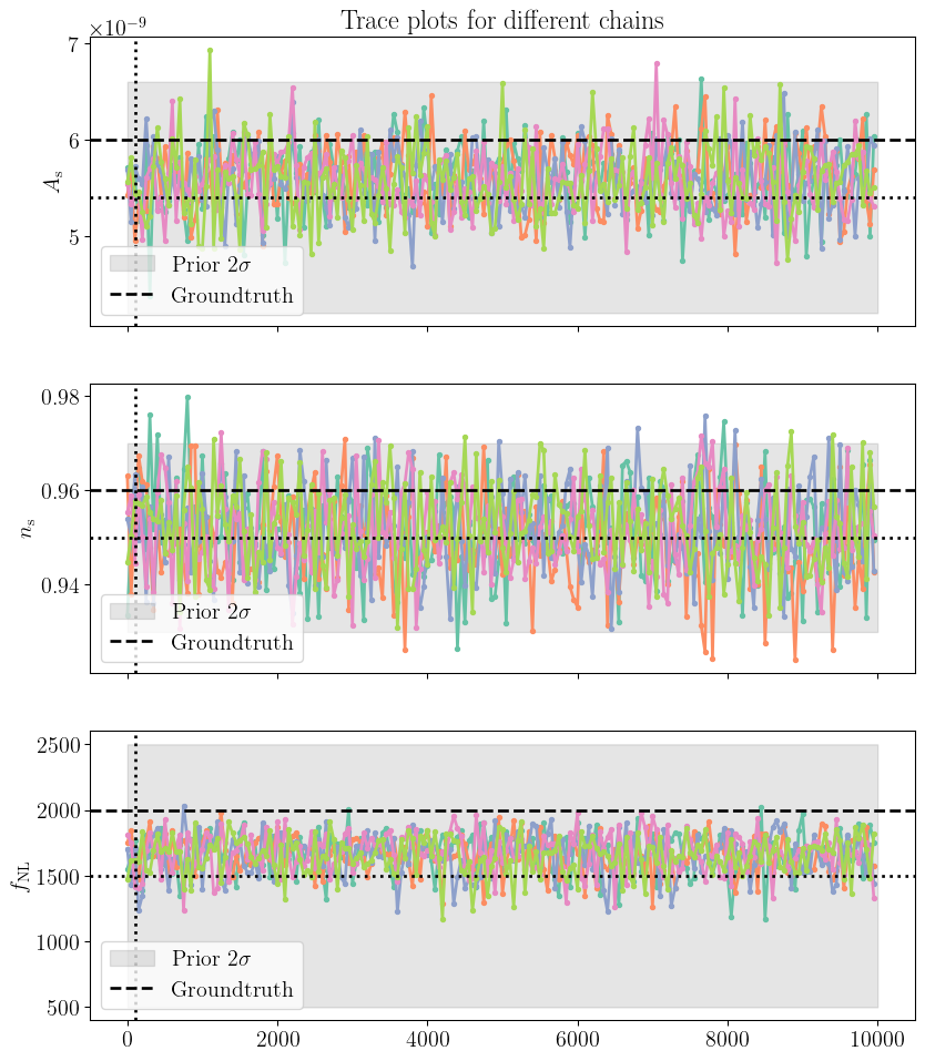
Figure 6: Trace plots for the cosmological parameters \(A_\mathrm{s}\), \(n_\mathrm{s}\), and \(f_\mathrm{NL}\) for each chain. The dashed line indicates the groundtruth value and the shaded area the \(2\sigma\) region of the Gaussian prior.
Sequential posterior power spectrum
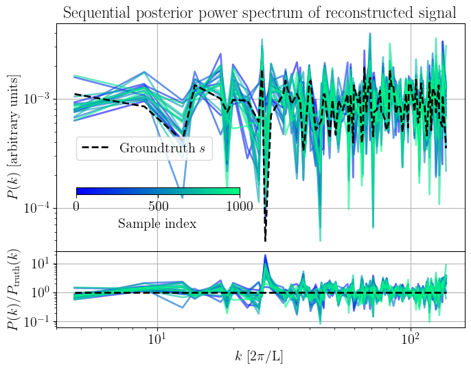
Given our samples, we can do posterior predictive checks to further ensure that the chain has converged to the correct posterior. To do so, one needs to run the data model using the samples as input. We perform posterior predictive cheks by looking at the power spectrum of the reconstructred signal and the ground truth. In practice, the groundtruth signal will not be available but we can compare against perturbation theory predictions.
Figure 7: Sequential posterior power spectrum of the reconstructed signal. The dashed line indicates the groundtruth power spectrum.
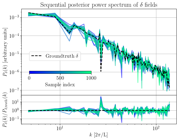
Figure 8: Sequential posterior power spectrum of the reconstructed \(\delta\) field. The dashed line indicates the groundtruth power spectrum of the \(\delta\) field.
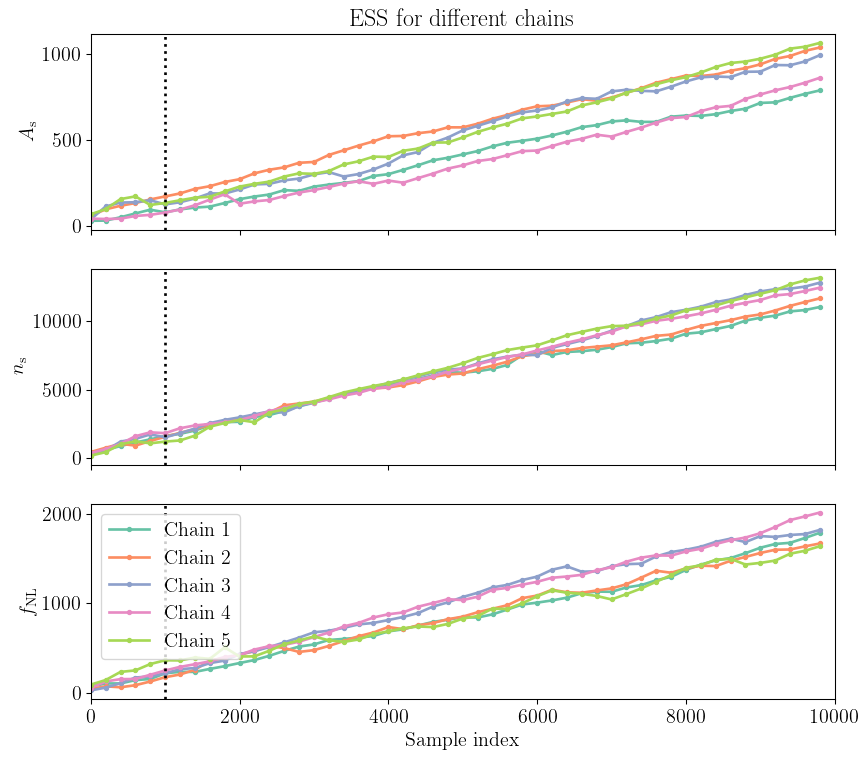
Effective sample size in the chains
When running an MCMC, samples are not independent. The effective sample size (ESS) is a measure of how many independent samples we have in our MCMC chain. It can be computed using the integrated autocorrelation time, which quantifies the correlation between samples at different lags. We here compute the ESS using function available in the emcee documentation. As the error of an MCMC estimator reduces with the number of samples, it is important to have a sufficiently large ESS.
Figure 9: Effective sample size (ESS) for the pixels (10, 20) and (25, 10) in the field for each chain. The dashed line indicates the burn-in period.
Figure 10: Effective sample size (ESS) for the cosmological parameters \(A_\mathrm{s}\), \(n_\mathrm{s}\), and \(f_\mathrm{NL}\) for each chain. The dashed line indicates the burn-in period.
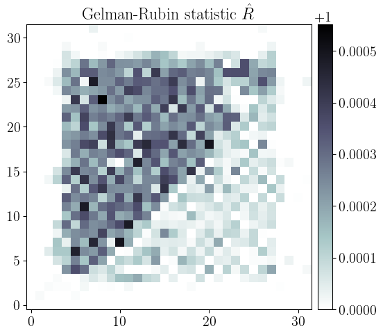
Gelman-Rubin test
Another useful test is the Gelman-Rubin (GR) test. It assess if the samples are uncorrelated by computing the ratio between the variance within the chains and between multiple independant chains.
Figure 11: Gelman-Rubin statistic \(\hat{R}\) for the field.
Visualise summaries of the chains
Now that we have carefully checked the convergence of the MCMC chains, we can visualise the results.
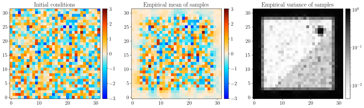
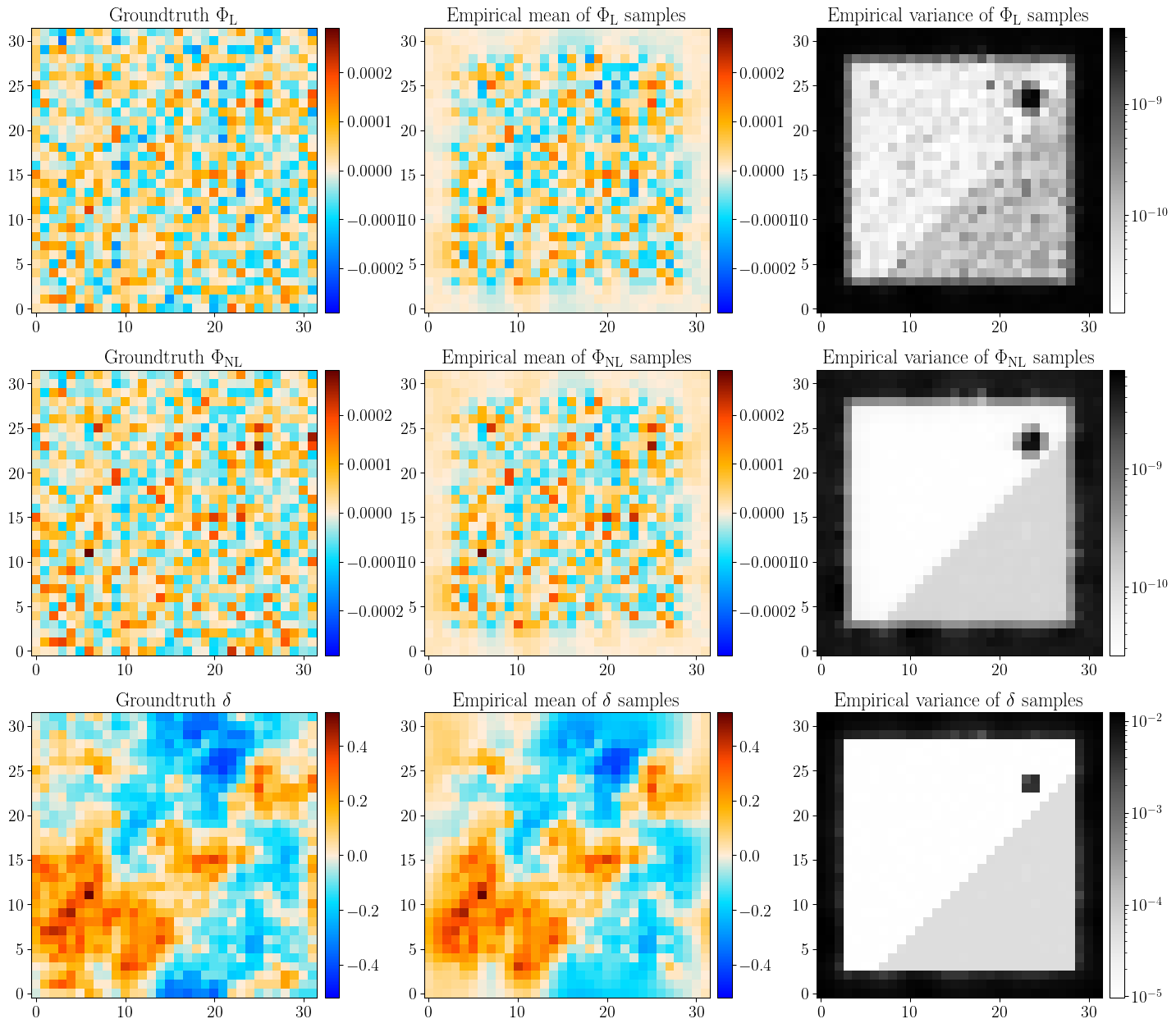
First, we can use the samples to reconstruct the \(\delta\) field and check that it visually matches the truth.
Figure 12: Reconstruction of the \(\Phi_\mathrm{L}\), \(\Phi_\mathrm{NL}\), and \(\delta\) fields from the initial conditions and cosmological parameters samples. The first row shows the initial conditions, the second row the groundtruth fields, the third row shows the empirical mean of the samples, and the fourth row shows the empirical variance of the samples.
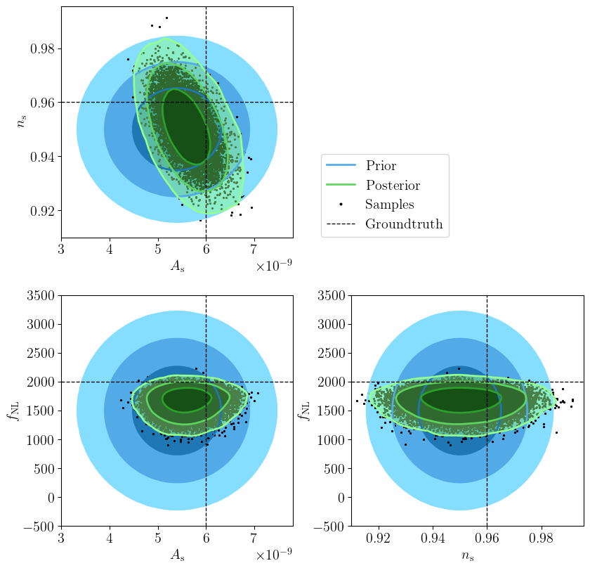
We can finally visualise the posterior samples in the cosmological parameters space.
Figure 13: Posterior samples in the cosmological parameters space. The blue contours show the prior distribution, while the green filled contours show the posterior distribution. The lines indicate the one, two, and three \(\sigma\) confidence level. The dashed lines indicate the groundtruth.
This result has been obtained sampling all latent variables. It is also possible to extract information at the field-level without relying on high-dimensional sampling of the initial conditions.